
Calculate a Sales Commission
November 26, 2021 - by Bill Jelen

Problem: The VP of sales in my company has dreamt up the most convoluted sales plan in the history of the world. Rather than just paying the reps a straight commission, this plan involves paying a base rate and a 2% bonus based on the product sold, and a monthly profit sharing bonus. For the spreadsheet below, I need to create a formula that can be copied to all rows and all months.
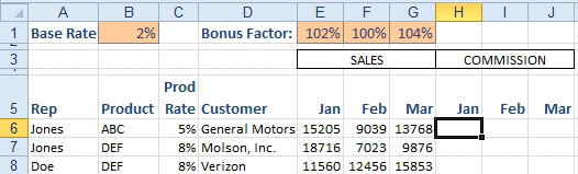
Strategy: This formula will contain all four reference types: relative, mixed, the other mixed, and absolute. While entering the first formula in H6, you want to base the commission calculation on the January sales in E6. As you copy the formula from January to February, you want the E6 reference to be able to change to F6. As you copy the formula down to other rows, you want the E6 to change to E7, E8, and so on. Thus, the E6 portion of the formula needs to be a relative reference and will have no dollar signs.
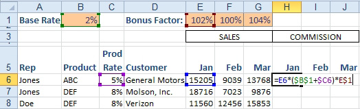
You multiply the sales by the base rate in B1. As you copy the formula to other months and rows, it always needs to point to B1. Thus, you need to use dollar signs before the B and before the 1: $B$1.
To incorporate the product bonus, you need to multiply sales by the product rate in column C. All the months in row 6 have to refer to C6. All the months in row 7 have to refer to C7. Thus, you need a mixed reference where column C is locked; use the address of $C6.
Finally, to address the monthly profit sharing bonus, the entire commission calculation is multiplied by the bonus factor shown in row 1. The January commission calculation uses the factor in E1. The February factor is in F1. The March factor is in G1. In this case, you need to allow the formula to point to different columns but always to row 1. This requires a mixed reference of E$1.
Now that you have the 4 components of the formula, enter this formula in E6: =E6*($B$1+$C6)*E$1.
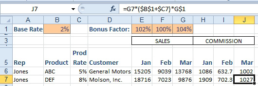
The concept of relative, absolute, and mixed references is one of the most important concepts in Excel. Being able to use the right reference will allow you to create a single formula that can be copied everywhere.
This article is an excerpt from Power Excel With MrExcel
Title photo by Sharon McCutcheon on Unsplash