
Calculate Workdays for 5, 6, and 7 Day Workweeks
January 22, 2021 - by Bill Jelen

Challenge: Calculate how many workdays fall between two dates. Excel’s NETWORKDAYS function does this if you happen to work the five days between Monday and Friday inclusive. This topic will show you how to perform the calculation for a company that works 5, 6, or 7 days a week.
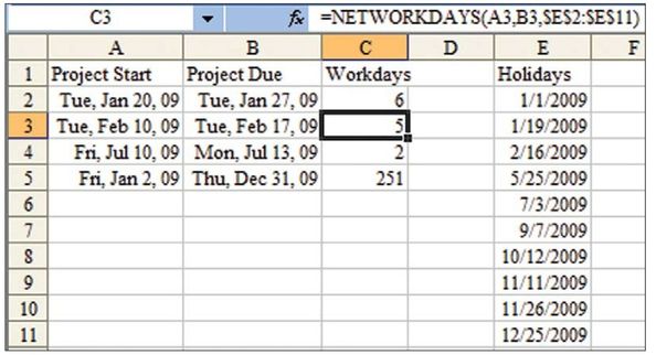
Background: The NETWORKDAYS function calculates the number of workdays between two dates, inclusive of the beginning and ending dates. You specify the earlier date as the first argument, the later date as the second argument, and optionally an array of holidays as the third argument. In Figure 2, cell C3 calculates only 5 workdays because February 16, 2009, is a holiday. This is a cool function, but if you happen to work Monday through Saturday, it will not calculate correctly for you.
Setup: Define a range named Holidays to refer to the range of holidays.
Solution: The formula in C3 is:
=SUMPRODUCT(--(COUNTIF(Holidays, ROW(INDIRECT(A3&":"&B3)))=0), --(WEEKDAY(ROW(INDIRECT(A3&":"&B3)),3)<6))
Although this formula deals with an array of cells, it ultimately returns a single value, so you do not need to use Ctrl+Shift+Enter when entering this formula.
Breaking It Down: The formula seeks to check two things. First, it checks whether any of the days within the date range are in the holiday list. Second, it checks to see which of the dates in the date range are Monday-through-Saturday dates.
You need a quick way to compare every date from A3 to B3 to the holiday list. In the current example, this encompasses only 8 days, but down in row 5, you have more than 300 days.
The formula makes use of the fact that an Excel date is stored as a serial number. Although cell A3 displays February 10, 2009, Excel actually stores the date as 39854. (To prove this to yourself, press Ctrl+‘ to enter Show Formulas mode. Press Ctrl+‘ to return to Normal mode.)
It is convenient that Excel dates in the modern era are in the 39,000 – 41,000 range, well within the 65,536 rows available in Excel 97-2003. The date corresponding to 65,536 is June 5, 2079, so this formula will easily continue to work for the next 70 years. (And if you haven’t upgraded to Excel 2007 by 2079, well, you have a tenacious IT department.)
Excel starts evaluating this formula with the first INDIRECT function. The arguments inside INDIRECT build an address that concatenates the serial number for the date in A3 with the serial number for the date in B3. As you can see in the sub-result, you end up with a range that points to rows 39854:39861:
Formula fragment: INDIRECT(A3&" : "&B3)
Sub-result: INDIRECT (“39854 : 39861”)
Normally, you would see something like “A2:IU2” as the argument for INDIRECT. However, if you have ever used the POINT method of entering a formula and gone from column A to the last column, you will recognize that =SUM(2:2) is equivalent to =SUM(A2:IV2) in Excel 2003 and =SUM(A2:XFD2) in Excel 2007.
The first step of the formula is to build a reference that is one row tall for each date between the start and end dates.
Next, the formula returns the ROW function for each row in that range. In the case of the dates in A3 and A4, the formula returns an array of eight row numbers (in this case, { 39854; 39855; 39856;…; 39861 } ). This is a clever way of returning the numbers from the first date to the last date. In row 5, the ROW function returns an array of 364 numbers:
Formula fragment: ROW(INDIRECT(A3&" : "&B3))
Sub-result: {39854;39855;39856;39857;39858;39859;39860;39861}
Now you can compare the holiday list to the range of dates. =COUNTIF(Holidays, sub-result) counts how many times each holiday is in the range of dates. In this case, you expect the function to return a 1 if a holiday is found in the range of dates and a 0 if the holiday is not found. Because you want to count only the non-holiday dates, the formula compares the COUNTIF result to find the dates where the holiday COUNTIF is 0:
Formula fragment: --COUNTIF(Holidays, ROW(INDIRECT(A3&":"&B3)))=0
Result: {1;1;1;1;1;1;0;1;1}
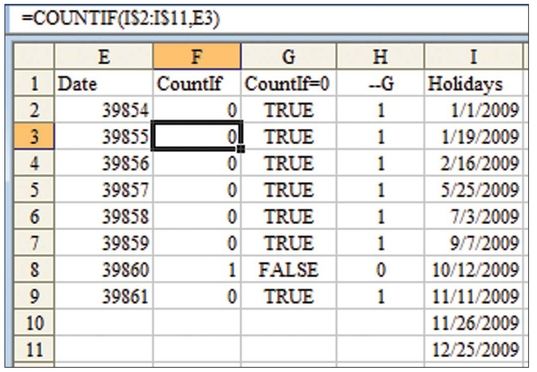
For every date in the date range, the COUNTIF formula asks, “Are any of the company holidays equal to this particular date?” Figure 3 illustrates what is happening in the first half of the formula. Column E represents the values returned by the ROW function. Column F uses COUNTIF to see if any of the company holidays are equal to the value in column E. For example, in E3, none of the holidays are equal to 39855, so COUNTIF returns 0. However, in F8, the formula finds that one company holiday is equivalent to 39860, so COUNTIF returns 1.
In column G, you test whether the result of the COUNTIF is 1. If it is, the TRUE says to count this day.
In column H, the minus-minus formula converts each TRUE value in column G to 1 and each FALSE value in column G to 0.
In Figure 3, cells H2:H9 represent the virtual results of the first half of the formula, which finds the dates that are not holidays.
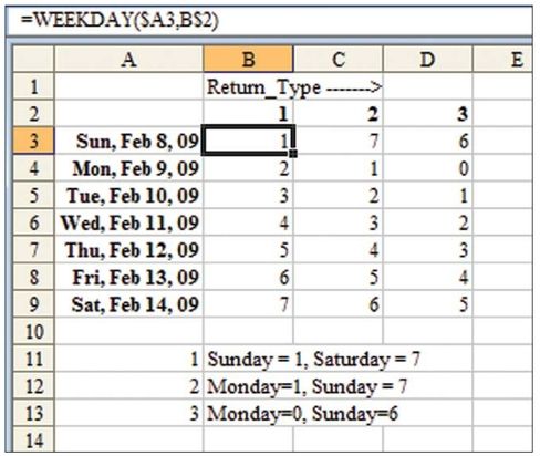
The second half of the formula uses the WEEKDAY function to find which dates are not Sundays. The WEEKDAY function can return three different sets of results, depending on the value passed as the Return Type argument. Figure 4 show the values returned for various Return Type arguments. In order to isolate Monday through Saturday, you could check to see if the WEEKDAY function with a Return Type of 1 is greater than 1. You could check to see if the WEEKDAY function with a Return Type of 2 is less than 7. You could check to see if the WEEKDAY function with a Return Type of 3 is less than 6. All these methods are equivalent.
The second half of the formula uses many of the tricks from the first half. The INDIRECT function returns a range of rows. The ROW function converts those rows to row numbers that happen to correspond to the range of dates. The WEEKDAY(,3) function then converts those dates to values from 0 to 6, where 6 is equivalent to Sunday. The virtual result of the WEEKDAY function is shown in column L of Figure 5. The formula compares the WEEKDAY result to see if it is less than 6. This virtual result is shown in column M of Figure 5. Finally, a double minus converts the TRUE/FALSE values to 0s and 1s, as shown in column N. Basically, this says that we are working every day in the range, except for N7, which is a Sunday.
Formula fragment: --(WEEKDAY(ROW(INDIRECT(A3&":"&B3)),3)<6)
Result: {1;1;1;1;1;1;0;1}
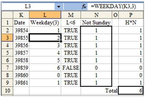
Finally, SUMPRODUCT multiplies the Not Holiday array by the Not Sunday array. When both arrays contain a 1, we have a workday. When either the Not Holiday array has a 0 (as in row 8) or the Not Sunday array has a 0 (as in row 7), the result is a 0. The final result is shown in the SUM function in P10: There are 6 workdays between the two dates.
As with most array solutions, this one formula manages to do a large number of sub-calculations to achieve a single result.
Additional Details: What if you work 7 days a week but want to exclude company holidays? The formula is simpler:
=SUMPRODUCT(--(COUNTIF(Holidays, ROW(INDIRECT(A2&":"&B2)))=0))
The problem becomes trickier if days in the middle of the week are the days off. Say that you have a part-time employee who works Monday, Wednesday, and Friday. The Not Sunday portion of the formula now needs to check for 3 specific weekdays. Note that the Return Type 2 version of the WEEKDAY function never returns a 0. Because this version of the WEEKDAY function returns digits 1 through 7, you can use it as the first argument in the CHOOSE function to specify which days are workdays. Using =CHOOSE(WEEKDAY(Some Date,2),1,0,1,0,1,0,0) would be a way of assigning 1s to Monday, Wednesday, and Friday.
Because CHOOSE does not usually return an array, you have to enter the following formula, using Ctrl+Shift+Enter:
=SUMPRODUCT(--(COUNTIF(Holidays, ROW(INDIRECT(A3&":"&B3)))=0), --(CHOOSE(WEEKDAY(ROW(INDIRECT(A3&":"&B3)),2),1,0,1,0,1,0,0)))
Summary: This topic introduces the concept of creating a huge array from two simple values. For example, =ROW(INDIRECT(“1:10000”)) generates a 10,000-cell array filled with the numbers from 1 to 10,000. You can use this concept to test many dates while only specifying a starting and ending point, thus solving the NETWORKDAYS problem for any type of workweek.
Source: "6 day work week with workday function?????" on the MrExcel Message Board.
Title Photo: Jazmin Quaynor at Unsplash.com
This article is an excerpt from Excel Gurus Gone Wild.