Customizing the Ribbon

July 15, 2021 - by Bill Jelen

Problem: I want to customize the ribbon.

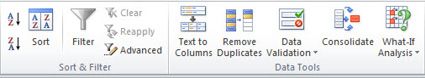
Strategy: Ribbon customizations in Excel are weak compared with the customization capabilities in Excel 2003. You might feel like the Pivot Table command belongs on the Data tab rather than on the Insert tab. You can add a new group to the Data tab to hold the pivot table icons. First, look at the ribbon and decide where you want the new group to appear. Perhaps a good location would be between the Sort & Filter group and the Data Tools group.

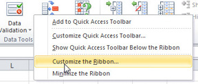
Detail of the Data tab in the Ribbon before customizing. Sort & Filter is a group on the left. Data Tools is a group on the right. — Figure 10. Decide where you want the new group to appear.

Right-click anywhere on the ribbon and choose Customize the Ribbon.

RIght-click anywhere in the Ribbon. The fourth choice is Customize the Ribbon. — Figure 11. Right-click the ribbon to access this menu.

The Customize dialog contains two large list boxes. You will first be working with the list box on the right side of the screen. Expand the plus sign next to the Data entry to see the groups on the Data tab. If you want a new group to appear after the Sort & Filter group, click Sort & Filter, and then click the New Group button below the list box.

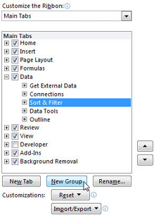
Expand the Data tab. Click on Sort & Filter and then New Group to add an empty group to the right of Sort & Filter. — Figure 12. Choose where the new group should go.

Excel adds a new group with the name of New Group (Custom). Click the Rename button below the list box.

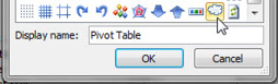
The new group is called "New Group (Custom)". Click the Rename button. — Figure 13. Choose to rename the group

Type a new name in the Rename dialog. Also, choose an icon. This icon will appear only when the Excel window gets small enough to force the group into a dropdown, as shown later in Figure 18.

Type a new name of Pivot Table — Figure 14. Type a new name and choose an icon to represent the group.

Note: The 180 icons available are a far cry from the 4096 icons available in Excel 2003. As I pointed out at the beginning of this chapter, toolbar customization took a giant step backward after Excel 2003.

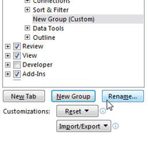
After renaming the new group in the list box on the right side, it is time to turn your attention to the list box on the left side. It starts out showing Popular Commands. Use the dropdown above the left list box to change from Popular Commands to All Commands.

Scroll down to the commands starting with Pivot. You will see a confusing array of commands. Click the first PivotTable icon, and click the Add button in the center of the screen. Click the second PivotChart icon, and then click the Add button. Click PivotTable and PivotChart Wizard, and then click the Add button.

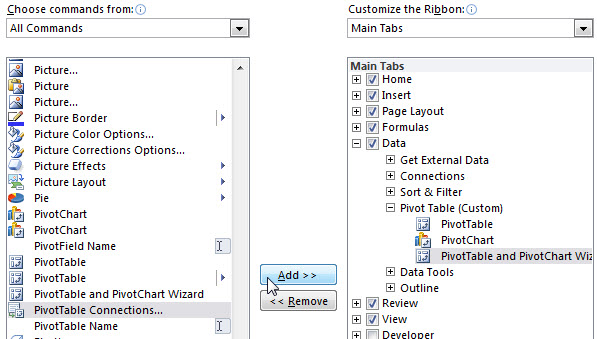
With the new Pivot Table (Custom) group selected, find commands on the left side and choose the Add>> button in the middle to add commands to the group. — Figure 15. Choose icons to add to the new group.

It is sometimes difficult to figure out which icons you want. There are two icons that say PivotTable. The first icon is simply an icon. The second icon is an icon with a rightward-facing triangle on the right side of the list box. That triangle indicates that the second icon is actually a dropdown that leads to more choices. That second PivotTable dropdown icon is the icon at the bottom half of the Insert tab’s Pivot Table group. It opens to enable you to choose between PivotTable and PivotChart. You might prefer to use that icon instead.

Two PivotChart icons are available. Hover over each icon to see that the first one is the PivotChart icon available on the PivotTable Tools Options tab. You will also see that the second icon is the one on the Insert tab. The first PivotChart icon will be grayed out unless you are in a pivot table. The second PivotChart icon is the one that is used to create a new pivot chart from a data set.

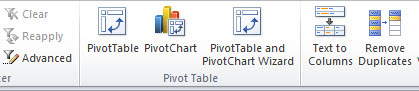
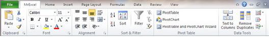
This figure shows the resulting group on the Data tab.

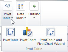
Success! The Pivot Table group offers Pivot Table, Pivot Chart, and the legacy Pivot Table and Pivot Chart Wizard. — Figure 16. The custom group is added to the ribbon.

If you are wondering why you had to choose an icon back in Figure 14, it is for people who have the Excel window resized to a narrower width. If you make your Excel window narrower, the custom group will eventually get squished down to a single dropdown. Your icon will appear on that dropdown, as shown here.

When you created the custom group, you chose an icon. If the Excel window shrinks and your group gets shrunk to a single icon, the icon you chose will decorate the drop-down menu. — Figure 17. The icon from Figure 14 shows with a smaller window size.

Note back in Figure 10 that the Sort icon appears as a large icon with a caption and that the AZ and ZA icons appear as small icons without a caption. How can you specify that the pivot table icon should be large and the pivot chart and wizard icons should be small? You can’t. At least not with the Excel interface.

If you want to start writing some XML and VBA, you can gain control over the size and images used in the ribbon. For an excellent book on this daunting task, look for RibbonX: Customizing the Office 2007 Ribbon by Robert Martin, Ken Puls and Teresa Hennig. Or, check out the Ribbon Commander utility described at http://mrx.cl/2dbS4Js.

I find that I spend most of my time on either the Home or the Data tab. If I could combine the left side of the Home tab with the right side of the Data tab, plus pivot tables, I would probably be able to spend all my time on one tab.

This figure shows a new MrExcel tab that reuses groups from other ribbon tabs to build a new tab.

A new MrExcel tab appears in the Ribbon, between the File and Home tabs. It offers formatting icons, plus pivot tables, sort, and remove duplicates. — Figure 18. The MrExcel tab is a custom tab with my favorite groups.

The general steps for creating a new ribbon tab are as follows:

1. Right-click the Ribbon and choose Customize the Ribbon.
2. Click New Tab at the bottom right of the dialog.
3. Click Rename and give the tab a name.
4. Use the Up and Down buttons at the right side of the dialog to move the new tab into the proper location.
5. From the left dropdown, choose Main Tabs.
6. In the left dropdown, expand an existing tab and find an existing group that you want to add to your new tab. Click that group and click Add.
7. Repeat step 6 to add additional groups.
8. You can reuse a custom group that you created previously. In the left dropdown, choose Custom Tabs and Groups. You can move the Pivot Table (Custom) tab created earlier in this chapter onto your new ribbon tab.
9. Click OK to finish customizing the ribbon tab.

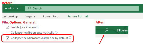
Problem: Why is the Search box so large? I never use this.

Strategy: Starting in the spring of 2019, you can collapse it to a small icon. Use File, Options, General

The Tell Me search box is taking up way too much space in the Excel title bar. If you go to File, Options, General and choose Collapse the Microsoft Search Box by Default, it reduces in size to a small magnifying glass icon. — Figure 9. Collapse the Search Box to a tiny icon.

This article is an excerpt from Power Excel With MrExcel

Title photo by Jess Bailey on Unsplash