Display Up/Down Arrows

March 23, 2022 - by Bill Jelen

Problem: I have a series of closing stock prices. If the price for the day goes up, I want to display an up symbol. If the price goes down, display a down symbol.

Strategy: Use an IF statement in combination with a Webdings or Wingdings font.

Most computers have at least four font faces composed of symbols. To easily browse the symbols, enter =CHAR(ROW()) in cells A1:A256. Change the font for column A to Webdings or one of the three Wingdings fonts. As you browse through the symbols and see one that you would like, click on the symbol. Below is a possible arrow to use. You can see that this is in the Wingdings 3 font. From the row number, you know it is character code 199. From the formula bar, you can see that it is the C with a cedilla mark below.

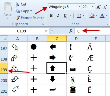
Character 199 in Wingdings3 font is an upward-pointing arrow. — Figure 392. Character 199 is a possibility.

If you are reading this and you have a Portuguese keyboard, you probably have a key with the cedilla C. However, you will have to fly to France to find an E with a grave accent. You could try to master the art of holding down Alt while typing 0199 on the numeric keypad, or you could use CHAR(199).

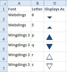
Personally, for me, all of those are too much hassle and I won’t use the arrows shown above. Instead, I found the symbols that correspond to letters on my keyboard, so that I can easily type them in the formula.

The number 6 in Webdings font is a triangle pointing down. The lower case p in Wingdings3 font is a larger triangle pointing up. Lower case r in Wingdings 3 is an outline of a triangle pointing up. — Figure 393. These six symbols are all typeable on a U.S. keyboard.

The strategy is to write an IF statement that produces a 5 for positive and a 6 for negative. Then, format those cells to use the Webdings font.

Use a formula such as =IF(B2>B3,5,6) to use the Webdings symbols. If you prefer the filled triangles from Wingdings 3, use =IF(B2>B3,”p”,”q”). Initially, you will get a column of 5 and 6.

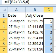
Dates in A are sorted with most recent at the top. Closing stock prices are in B. The formula in C2 is =IF(B2>B3,5,6) and produces a column of 5 or 6. — Figure 394. The formula produces 5’s and 6’s.

Select column C and change the font to Webdings. Use Left alignment.

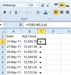
When you change those 5's or 6's to Webdings font, you get triangles pointing up or down. — Figure 395. Convert the column to Wingdings.

Gotcha: If you ever need to edit the formula in C, it will appear in Webdings font and be unreadable in the cell. Use the Formula bar to see the real formula.

If you want to display the arrows in green and red, change the font color of column C to green. Then use Home, Conditional Formatting, Highlight Cells Rules, Equal to, 5. Open the Format dropdown and choose Custom Format. On the Font tab, choose a bright red.

While Wingdings is a cool technique, an easier way to display Up/Down Arrows is "Use the SIGN Function for Up/Flat/Down Icon Set" on page 522

Alternate Strategy: You can avoid the IF statement and use a custom number format. Use a formula of =SIGN(B2-B3) in column C. This will return a negative one for days that the price went down, positive one for days when the price went up, and a zero for days where the price is unchanged.

Change the custom number format to [green]\r;[red]\s;. Change the font to Wingdings 3.

Same stock prices and dates as in the last example. This time, the formula is =SIGN(B4-B5) and is either positive 1 or negative 1. The Custom Number Format uses two zones: [Green]\r;[Red]\s; When shown in Wingdings3 font, you get a green triangle pointing up for increases and a red triangle pointing down for decreases. — Figure 396. Forcing Excel to show r for positive and s for negative.

The custom number format is using three zones. The first zone is showing a lower case r in green for any positive number. The second zone is showing a lower case s in red for any negative number. The third zone is indicated by the final semi-colon and is blank, indicating no symbol for zero values. When you convert column C to Wingdings 3, you get the arrows shown.

This article is an excerpt from Power Excel With MrExcel

Title photo by Susan Q Yin on Unsplash