Dynamic Arrays: Formulas Can Now Spill

August 10, 2022 - by Bill Jelen

Let's start with the basic array formula. Go to cell E3. Type =A2:C10, as shown here. In the past, you would have had to wrap that formula in an aggregation function and maybe use Ctrl+Shift+Enter.

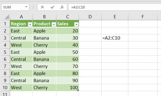
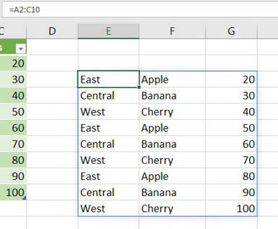
Three columns of data in A2:C10. Off to the right, you are about to enter a formula of =A2:C10 in cell E3. — Figure 605. One cell, pointing to many cells.

But now you can simply press Enter. Excel returns 27 answers—and the answers spill into the adjacent cells! Look at the formula in the formula bar...there aren’t any curly braces, which means no one pressed Ctrl+Shift+Enter.

The one formula =A2:C10 returns a three-column by 9-row set of results. The formula bar shows =A2:C10. A green outline appears around the entire results set. — Figure 606. One formula brought all of these answers.

Note: If you type a new row in A11:C11, the formula automatically expands to include the extra row.This happened because A1:C10 is defined as a Ctrl+T table. It would also happen if you inserted new rows in the middle of a regular range.

While Dynamic Array formulas can point to a table, you cannot include Dynamic Array results in a table.

How will you ever refer to E3:G13 if you don't know how tall the range is going to be? For this, you add the spilled range operator (#) after the cell containing the array formula.

For example, =E3 refers to Apple. =E3# refers to the entire array that starts in E3. This is unofficially called Array Reference notation.

Note that the Array Reference notation is not supported when linking to an external workbook.

Since the # mops up all of the spilled cells, Ingeborg Hawighorst suggested naming it The Spiller.

This article is an excerpt from Power Excel With MrExcel

Title photo by Praveen kumar Mathivanan on Unsplash