Excel 2020: Compare Budget Versus Actual via Power Pivot

June 22, 2020 - by Bill Jelen

Compare Budget Versus Actual via Power Pivot. Photo Credit: Michael Longmire at Unsplash.com

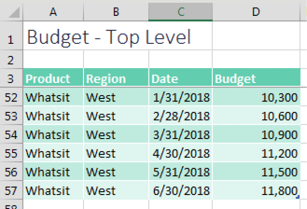
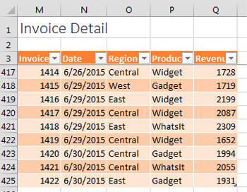
Budgets are done at the top level – revenue by product line by region by month. Actuals accumulate slowly over time – invoice by invoice, line item by line item. Comparing the small Budget file to the voluminous Actual data has been a pain forever. I love this trick from Rob Collie, aka PowerPivotPro.com.

To set up the example, you have a 54-row budget table: 1 row per month per region per product.

The Budget table is four columns and 54 rows: Product, Region, Date, Budget.

The invoice file is at the detail level: 422 rows so far this year.

The Invoice table has a thousand rows. Columns ar Invoice, Date, Region, Product, Customer.

There is no VLOOKUP in the world that will ever let you match these two data sets. But, thanks to Power Pivot (aka the Data Model in Excel 2013+), this becomes easy.

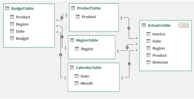
You need to create tiny little tables that I call “joiners” to link the two larger data sets.

A cartoon shows a big ugly mean Actuals sitting at a table with a tiny meek Budget. They won't get along. But in the middle, trying to talk to both of them are three tiny joiner tables. — Illustration: George Berlin

In my case, Product, Region, and Date are in common between the two tables. The Product table is a tiny four-cell table. Ditto for Region. Create each of those by copying data from one table and using Remove Duplicates.

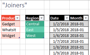
The three joiner tables. The Product table is a Product heading and three rows by 1 column: Gadget, WhatsIt and Widget. The Region table is a Region heading and three rows of Central, East, West. The Calendar table is larger. It has two columns: Date and Month. It continues beyond the edge of the figure, including every date found in either table.

The calendar table on the right was actually tougher to create. The budget data has one row per month, always falling on the end of the month. The invoice data shows daily dates, usually weekdays. So, I had to copy the Date field from both data sets into a single column and then remove duplicates to make sure that all dates are represented. I then used =TEXT(J4,"YYYY-MM") to create a Month column from the daily dates.

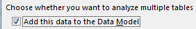
If you don’t have the full Power Pivot add-in, you need to create a pivot table from the Budget table and select the checkbox for Add This Data to the Data Model.

As you create the pivot table, choose the box for Add This Data To The Data Model.

As discussed in the previous tip, as you add fields to the pivot table, you will have to define six relationships. While you could do this with six visits to the Create Relationship dialog, I fired up my Power Pivot add-in and used the diagram view to define the six relationships.

You will be creating six relationships. Create three relationships from the Budget table to the three joiner tables. Create three relationships from the Actuals table to the three joiner tables.

Here is the key to making all of this work: You are free to use the numeric fields from Budget and from Actual. But if you want to show Region, Product, or Month in the pivot table, they must come from the joiner tables!

Here is a pivot table with data coming from five tables. Column A is coming from the Region joiner. Row 2 is coming from the Calendar joiner. The Product slicer is from the Product joiner. The Budget numbers come from the Budget table, and the Actual numbers come from the Invoice table.

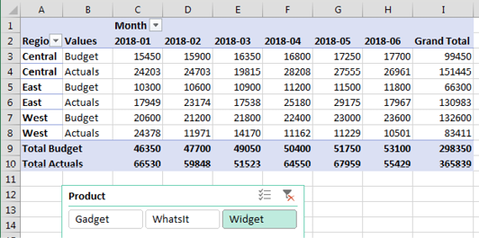
This pivot table has Region and Budget/Actual down the side. Months across the top. A Product slicer at the bottom.

This works because the joiner tables apply filters to the Budget and Actual table. It is a beautiful technique and shows that Power Pivot is not just for big data.

Title Photo: Michael Longmire at Unsplash.com

This article is an excerpt from MrExcel 2020 - Seeing Excel Clearly.