Excel 2020: Create a Year-over-Year Report in a Pivot Table

May 04, 2020 - by Bill Jelen

Let’s say you have two years’ worth of detail records. Each record has a daily date. When you build a pivot table from this report, you will have hundreds of rows of daily dates in the pivot table. This is not much of a summary.

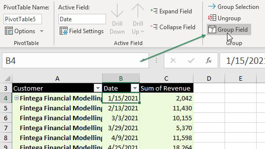
Choose one of those date cells in the pivot table. From the Analyze tab in the Ribbon, choose Group Field.

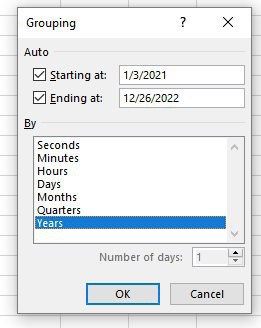
Because you are on a date field, you get this version of the Grouping dialog. In it, deselect Months and select Years.

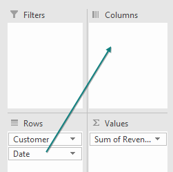
The daily dates are rolled up to years. Move the Date field from Rows to Columns.

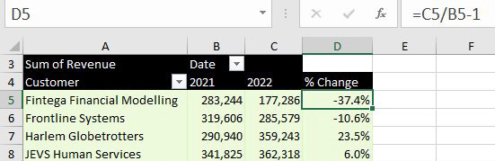
The result is almost perfect. But instead of a grand total in column D, you probably want a percentage variance. To get rid of the Grand Total column, right-click on the Grand Total heading and choose Remove Grand Total.)

To build the variance column as shown below, you need to write a formula outside the pivot table that points inside the pivot table. Do not touch the mouse or arrow keys while building the formula, or the often-annoying GETPIVOTDATA function will appear. Instead, simply type =C5/B5-1 and press Enter.

Title Photo: Henry & Co at Unsplash.com

This article is an excerpt from MrExcel 2020 - Seeing Excel Clearly.