Excel 2020: Eliminate VLOOKUP with the Data Model

June 17, 2020 - by Bill Jelen

Eliminate VLOOKUP with the Data Model. Photo Credit: Fredy Jacob at Unsplash.com

Say that you have a data set with product, date, customer, and sales information.

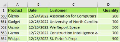
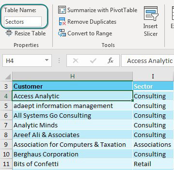
A data set wth Product, Date, Customer, and Quantity.

The IT department forgot to put sector in there. Here is a lookup table that maps customer to sector. Time for a VLOOKUP, right?

A second data set is a lookup table, mapping Customer to Industry Sector. Both data sets should be formatted as a table using Ctrl+T. Use the Table Name box on the Table Tools tab of the Ribbon to assign a name such as Sectors to this table.

There is no need to do VLOOKUPs to join these data sets if you have Excel 2013 or newer. These versions of Excel have incorporated the Power Pivot engine into the core Excel. (You could also do this by using the Power Pivot add-in for Excel 2010, but there are a few extra steps.)

In both the original data set and the lookup table, use Home, Format as Table. On the Table Tools tab, rename the table from Table1 to something meaningful. I’ve used Data and Sectors.

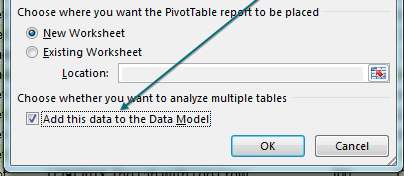
Select one cell in the data table. Choose Insert, Pivot Table. Starting in Excel 2013, there is an extra box, Add This Data to the Data Model, that you should select before clicking OK.

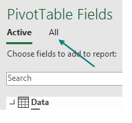
As you create the pivot table, the last choice in the Create PivotTable dialog is Add This Data To The Data Model.

The Pivot Table Fields list appears, with the fields from the Data table. Choose Revenue. Because you are using the Data Model, a new line appears at the top of the list, offering Active or All. Click All.

Surprisingly, the PivotTable Fields list offers all the other tables in the workbook. This is ground-breaking. You haven’t done a VLOOKUP yet. Expand the Sectors table and choose Sector. Two things happen to warn you that there is a problem.

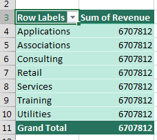
The PivotTable Fields pane now offers a choice at the top for Active, or All.

First, the pivot table appears with the same number in all the cells.

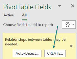
Something is wrong. Every industry sold exactly $6.7 Million.

Perhaps the more subtle warning is a yellow box that appears at the top of the PivotTable Fields list, indicating that you need to create a relationship. Choose Create. (If you are in Excel 2010 or 2016, try your luck with Auto-Detect - it often succeeds.)

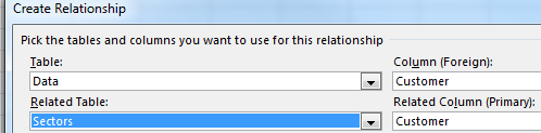
A yellow warning at the top of the PivotTable Fields says "Relationship Between Tables May Be Needed". Choose Auto-Detect or Create.

In the Create Relationship dialog, you have four dropdown menus. Choose Data under Table, Customer under Column (Foreign), and Sectors under Related Table. Power Pivot will automatically fill in the matching column under Related Column (Primary). Click OK.

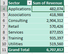
There are four settings to define a relationship. The table called Data has a field called Customer. The Related Table called Sectors has a field called Customer.

The resulting pivot table is a mash up of the original data and the data in the lookup table. No VLOOKUPs required.

The pivot table is now reporting Sector from Sheet2 and Revenue from Sheet1, thanks to the Data Model and the Relationship.

Title Photo: Fredy Jacob at Unsplash.com

This article is an excerpt from MrExcel 2020 - Seeing Excel Clearly.