Excel 2020: See Why GETPIVOTDATA Might Not Be Entirely Evil

June 15, 2020 - by Bill Jelen

Most people first encounter GETPIVOTDATA when they try to build a formula outside a pivot table that uses numbers in the pivot table. For example, this variance percentage won’t copy down to the other months due to Excel inserting GETPIVOTDATA functions.

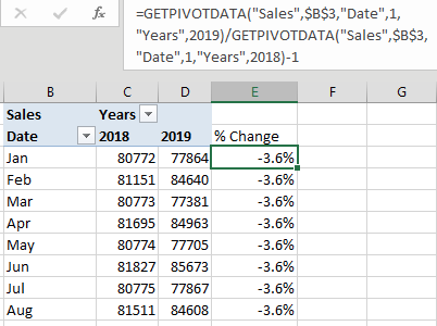
Excel inserts GETPIVOTDATA any time you use the mouse or arrow keys to point to a cell inside the pivot table while building a formula outside the pivot table.

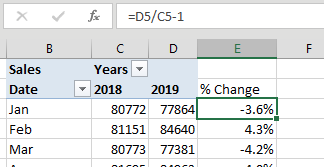
By the way, if you don’t want the GETPIVOTDATA function to appear, simply type a formula such as =D5/C5-1 without using the mouse or arrow keys to point to cells. That formula copies without any problems.

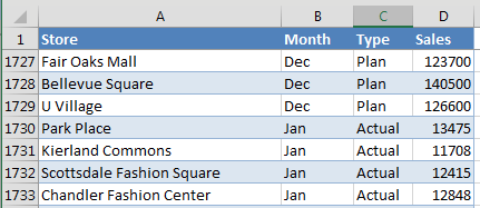
Here is a data set that contains one plan number per month per store. There are also actual sales per month per store for the months that are complete. Your goal is to build a report that shows actuals for the completed months and plan for the future months.

Build a pivot table with Store in Rows. Put Month and Type in Columns. You get the report shown below, with January Actual, January Plan, and the completely nonsensical January Actual+Plan.

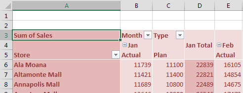
If you select a month cell and go to Field Settings, you can change Subtotals to None.

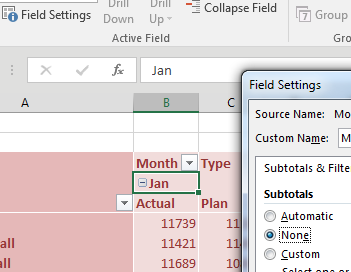
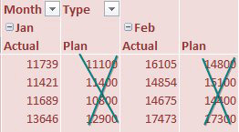
This removes the useless Actual+Plan. But you still have to get rid of the plan columns for January through April. There is no good way to do this inside the pivot table.

So, your monthly workflow becomes:

1. Add the actuals for the new month to the data set.
2. Build a new pivot table from scratch.
3. Copy the pivot table and paste as values so it is not a pivot table anymore.
4. Delete the columns that you don’t need.

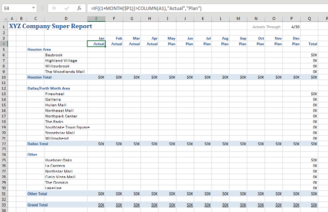
There is a better way to go. The following very compressed figure shows a new Excel worksheet added to the workbook. This is all just straight Excel, no pivot tables. The only bit of magic is an IF function in row 4 that toggles from Actual to Plan, based on the date in cell P1.

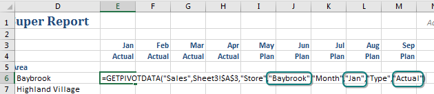
The very first cell that needs to be filled in is January Actual for Baybrook. Click in that cell and type an equal sign.

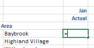
Using the mouse, navigate back to the pivot table. Find the cell for January Actual for Baybrook. Click on that cell and press Enter. As usual, Excel builds one of those annoying GETPIVOTDATA functions that cannot be copied.

But today, let’s study the syntax of GETPIVOTDATA.

The first argument below is the numeric field "Sales". The second argument is the cell where the pivot table resides. The remaining pairs of arguments are field name and value. Do you see what the auto-generated formula did? It hard-coded "Baybrook" as the name of the store. That is why you cannot copy these auto-generated GETPIVOTDATA formulas. They actually hard-code names into formulas. Even though you can‘t copy these formulas, you can edit them. In this case, it would be better if you edited the formula to point to cell $D6.

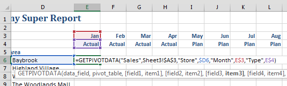
The figure below shows the formula after you edit it. Gone are "Baybrook", "Jan", and "Actual". Instead, you are pointing to $D6, E$3, and E$4.

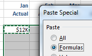
Copy this formula and then choose Paste Special, Formulas in all of the other numeric cells.

Now here‘s your monthly workflow:

1. Build an ugly pivot table that no one will ever see.
2. Set up the report worksheet.

Each month, you have to:

1. Paste new actuals below the data.
2. Refresh the ugly pivot table.

3. Change cell P1 on the report sheet to reflect the new month. All the numbers update.

   

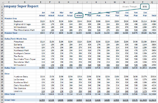
You have to admit that using a report that pulls numbers from a pivot table gives you the best of both worlds. You are free to format the report in ways that you cannot format a pivot table. Blank rows are fine. You can have currency symbols on the first and last rows but not in between. You get double-underlines under the grand totals, too.

Thanks to @iTrainerMX for suggesting this feature.

Title Photo: Manki Kim at Unsplash.com

This article is an excerpt from MrExcel 2020 - Seeing Excel Clearly.