
Excel 2020: Replace Columns of VLOOKUP with a Single MATCH
August 17, 2020 - by Bill Jelen

The following figure shows a situation in which you have to do 12 VLOOKUP functions for each account number.
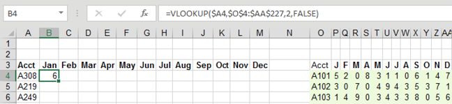
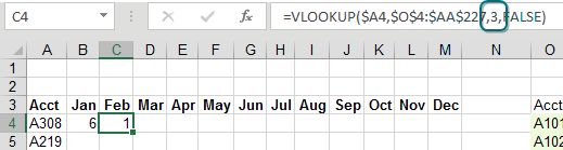
VLOOKUP is powerful, but it takes a lot of time to do calculations. Plus, the formula has to be edited in each cell as you copy across. The third argument has to change from 2 to 3 for February, then 4 for March, and so on.
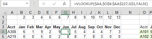
One workaround is to add a row with the column numbers. Then, the third argument of VLOOKUP can point to this row, as shown below. At least you can copy the same formula from B4 and paste to C4:M4 before copying the 12 formulas down.
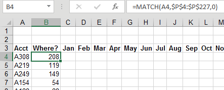
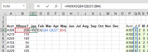
But here is a much faster approach: add a new column B with Where? as the heading. Column B contains a MATCH function. This function is very similar to VLOOKUP: You are looking for the value in A4 in the column P4:P227. The 0 at the end is like the False at the end of VLOOKUP. It specifies that you want an exact match. Here is the big difference: MATCH returns where the value is found. The answer 208 says that A308 is the 208th cell in the range P4:P227. From a recalc time perspective, MATCH and VLOOKUP are about equal.
I can hear what you are thinking: “What good is it to know where something is located? I’ve never had a manager call up and ask, ‘What row is that receivable in?’”
While humans rarely ask what row something is in, it can be handy for the INDEX function to know that position. The formula in the following figure tells Excel to return the 208th item from Q4:Q227.
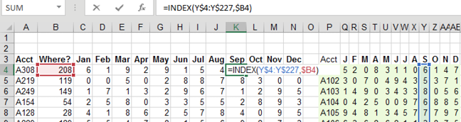
As you copy this formula across, the array of values moves across the lookup table as shown below. For each row, you are doing one MATCH and 12 INDEX functions. The INDEX function is incredibly fast compared to VLOOKUP. The entire set of formulas will calculate 85% faster than 12 columns of VLOOKUP.
Note
In late 2018, Office 365 introduced new logic for VLOOKUP that makes the calculation speed as fast as the INDEX/MATCH shown here.
Title Photo: Javier Reyes at Unsplash.com
This article is an excerpt from MrExcel 2020 - Seeing Excel Clearly.