
Excel 2020: Replace Nested IFs with a Lookup Table
August 27, 2020 - by Bill Jelen

A long time ago, I worked for the vice president of sales at a company. I was always modeling some new bonus program or commission plan. I became pretty used to commission plans with all sorts of conditions. The one shown in this tip is pretty tame.
The normal approach is to start building a nested IF formula. You always start at either the high end or the low end of the range. “If sales are over $500K, then the discount is 20%; otherwise,....” The third argument of the IF function is a whole new IF function that tests for the second level: "If sales are over $250K, then the discount is 15%; otherwise,....”
These formulas get longer and longer as there are more levels. The toughest part of such a formula is remembering how many closing parentheses to put at the end of the formula.
If you‘re using Excel 2003, your formula is already nearing the limit. With that version, you cannot nest more than 7 IF functions. It was an ugly day when the powers that be changed the commission plan and you needed a way to add an eighth IF function. Today, you can nest 64 IF functions. You should never nest that many, but it is nice to know there is no problem nesting 8 or 9.
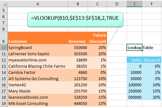
Rather than use the nested IF function, try using the VLOOKUP function. When the fourth argument of VLOOKUP changes from False to True, the function is no longer looking for an exact match. Well, first VLOOKUP tries to find an exact match. But if an exact match is not found, Excel settles into the row just less than what you are searching for.
Consider the table below. In cell C13, Excel will be looking for a match for $28,355 in the table. When it can’t find 28355, Excel will return the discount associated with the value that is just less—in this case, the 1% discount for the $10K level.
When you convert the rules to the table in E13:F18, you need to start from the smallest level and proceed to the highest level. Although it was unstated in the rules, if someone is below $10,000 in sales, the discount will be 0%. You need to add this as the first row in the table.
Caution
When you are using the “True” version of VLOOKUP, your table has to be sorted ascending. Many people believe that all lookup tables have to be sorted. But a table needs to be sorted only for an approximate match.
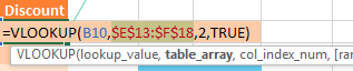
What if your manager wants a completely self-contained formula and does not want to see the bonus table off to the right? After building the formula, you can embed the table right into the formula. Put the formula in Edit mode by double-clicking the cell or by selecting the cell and pressing F2. Use the cursor to select the entire second argument: $E$13:$F$18.
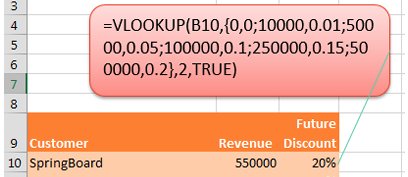
Press the F9 key. Excel embeds the lookup table as an array constant. In the array constant, a semicolon indicates a new row, and a comma indicates a new column. See Understanding Array Constants.

Press Enter. Copy the formula down to the other cells.
You can now delete the table. The final formula is shown below.
Thanks to Mike Girvin for teaching me about the matching parentheses. The VLOOKUP technique was suggested by Danny Mac, Boriana Petrova, Andreas Thehos, and @mvmcos.
Title Photo: Henrique Jacob at Unsplash.com
This article is an excerpt from MrExcel 2020 - Seeing Excel Clearly.