Excel 2020: Suppress Errors with IFERROR

September 02, 2020 - by Bill Jelen

Formula errors are common. If you have a data set with hundreds of records, a divide-by-zero and an #N/A errors are bound to pop up now and then.

In the past, preventing errors required Herculean efforts. Nod your head knowingly if you’ve ever knocked out =IF(ISNA(VLOOKUP(A2,Table,2,0),"Not Found",VLOOKUP(A2,Table,2,0)). Besides being really long to type, that solution requires twice as many VLOOKUPs. First, you do a VLOOKUP to see if the VLOOKUP is going to produce an error. Then you do the same VLOOKUP again to get the non-error result.

Excel 2010 introduced the greatly improved =IFERROR(Formula,Value If Error). I know that IFERROR sounds like the old ISERROR, ISERR, and ISNA functions, but it is completely different.

This is a brilliant function: =IFERROR(VLOOKUP(A2,Table,2,0),"Not Found"). If you have 1,000 VLOOKUPs and only 5 return #N/A, then the 995 that worked require only a single VLOOKUP. Only the 5 VLOOKUPs returned #N/A that need to move on to the second argument of IFERROR.

Oddly, Excel 2013 added the IFNA() function. It is just like IFERROR but only looks for #N/A errors. One might imagine a strange situation where the value in the lookup table is found, but the resulting answer is a division by 0. If you want to preserve the divide-by-zero error for some reason, you can use IFNA() to do this.

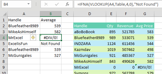
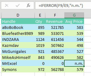
Of course, the person who built the lookup table should have used IFERROR to prevent the division by zero in the first place. In the figure below, the "n.m." is a former manager’s code for “not meaningful.”

Thanks to Justin Fishman, Stephen Gilmer, and Excel by Joe.

Title Photo: Anthony Ginsbrook at Unsplash.com

This article is an excerpt from MrExcel 2020 - Seeing Excel Clearly.