
Excel 2020: Use a Pivot Table to Compare Lists
May 27, 2020 - by Bill Jelen

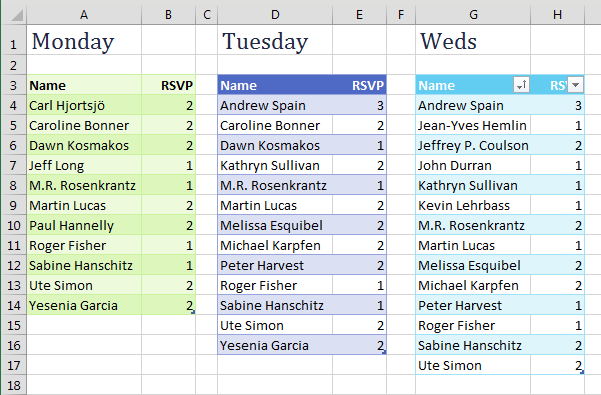
When you think of comparing lists, you probably think of VLOOKUP. If you have two lists to compare, you need to add two columns of VLOOKUP. In the figure below, you are trying to compare Tuesday to Monday and Wednesday to Tuesday and maybe even Wednesday to Monday. It is going to take a lot of VLOOKUP columns to figure out who was added to and dropped from each list.
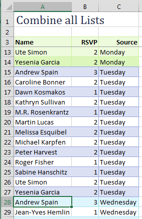
You can use pivot tables to make this job far easier. Combine all of your lists into a single list with a new column called Source. In the Source column, identify which list the data came from.
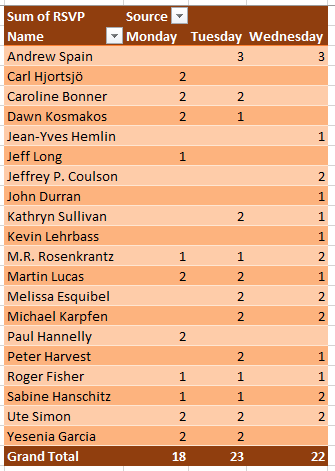
Build a pivot table from the combined list, with Name in rows, RSVP in values, and Source in columns. Turn off the Grand Total row, and you have a neat list showing a superset from day to day, as shown below.
Title Photo: Element5 Digital at Unsplash.com
This article is an excerpt from MrExcel 2020 - Seeing Excel Clearly.