Excel 2024: Create Your First Pivot Table

Pivot tables let you summarize tabular data to a one-page summary in a few clicks. Start with a data set that has headings in row 1. It should have no blank rows, blank columns, blank headings or merged cells.

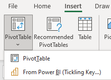
Select a single cell in your data and choose Insert, Pivot Table.

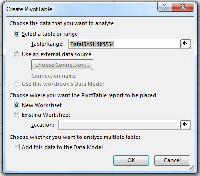
Excel will detect the edges of your data and offer to create the pivot table on a new worksheet. Click OK to accept the defaults.

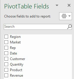
Excel inserts a new blank worksheet to the left of the current worksheet. On the right side of the screen is the Pivot Table Fields pane. At the top, a list of your fields with checkboxes.

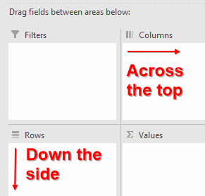
At the bottom are four drop zones with horrible names and confusing icons. Any fields that you drag to the Columns area will appear as headings across the top of your report. Any fields that you drag to the Rows area appear as headings along the left side of your report. Drag numeric fields to the Values area.

---

---

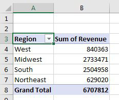
You can build some reports without dragging the fields. If you checkmark a text field, it will automatically appear in the Rows area. Checkmark a numeric field and it will appear in the Values area. By choosing Region and Revenue, you will create this pivot table:

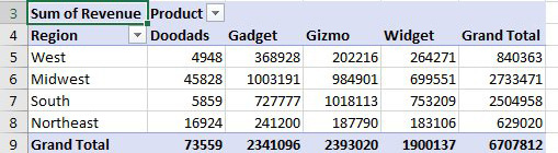
To get products across the top of the report, drag the Product field and drop it in the Columns area:

Bonus Tip: Rearrange fields in a pivot table

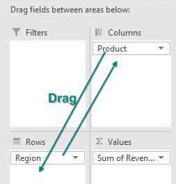
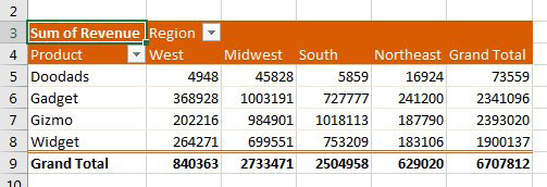
The power of pivot tables is the ability to rearrange the fields. If your manager decides you should put Regions across the top and products down the side, it is two drags to create the new report. Drag product to Rows. Drag Region to Columns.

You will have this report:

To remove a field from the pivot table, drag the field tile outside of the Fields pane, or simply uncheck the field in the top of the Fields pane.

Bonus Tip: Format a Pivot Table

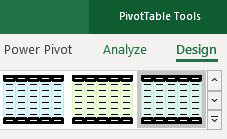
The Design tab has a gallery with 84 built-in formats for pivot tables. Choose a design from the gallery and the colors change.

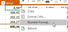
One frustrating feature with a pivot table is that the numbers always start out as General format. Right-click any number and choose Number Format…. Any changes you make to the number formatting using this command will be remembered as long as Revenue stays in the pivot table. (Before Excel 2010, pivot tables would frequently forget the number formatting. This was fixed in Excel 2010.)

Bonus Tip: Format One Cell in a Pivot Table

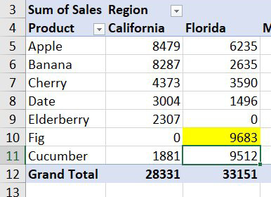
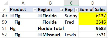
This is new in Microsoft 365 starting in 2018. You can right-click any cell in a pivot table and choose Format Cell. Any formatting that you apply is tied to that data in the pivot table. In the figure below, Florida Figs have a yellow fill color.

If you change the pivot table, the yellow formatting follows the Florida Fig.

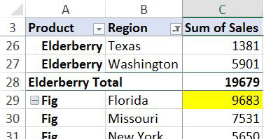
If you add a new inner field, then multiple cells for Florida Fig will have the fill color.

The formatting will persist if you remove Florida or Fig due to a filter. If you filter to vegetables, Fig is hidden. Filter to fruit and Fig will still be formatted. However, if you completely remove either Product or Region from the pivot table, the formatting will be lost.

Bonus Tip: Fill in the Blanks in the Annoying Outline View

If your pivot table is in Tabular or Outline Form and you have more than one row field, the pivot table defaults to leaving a lot of blank cells in the outer row fields: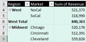

Starting in Excel 2010, use Design, Report Layout, Repeat all Item Labels to fill in the blanks in column A: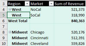

Bonus Tip: Replace Blank Values Cells With Zero

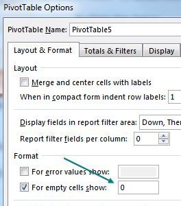
There is another way to have blanks in the Values area of a pivot table. Say that you have a product which is only sold in a few regions. If there are no Doodad sales in Atlanta, Excel will leave that cell empty instead of putting a zero there. Right-click the pivot table and choose Pivot Table Options. On the Layout & Format tab, find the box For Empty Cells, Show: and type a zero. Or, as Hunstville Excel Consultant Andrew Spain discovered, you can simply clear the checkbox to the left of For Empty Cells, Show:

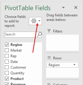
Bonus Tip: Rearrange Fields Pane Howie Dickerman was the Project Manager in charge of pivot tables at Microsoft. He inherited the product and suggests some of the defaults could have been different. For one, he suggests using the gear at the top right of the PivotTable Fields pane and changing the view to Fields Section and Areas Section side-by-side.