Excel 2024: Make Pivot Tables Expandable Using Ctrl+T


May 15, 2024 - by

Excel 2024: Make Pivot Tables Expandable Using Ctrl+T

If you choose all of columns A:J and you later want to add more records below the data, it takes only a simple Refresh to add the new data instead of having to find the Change Data Source icon. In the past, this made sense. But today, Change Data Source is right next to the Refresh button and not hard to find. Plus, there is a workaround in the Ctrl+T table.

When you choose your data set and select Format as Table by using Ctrl+T, the pivot table source will grow as the table grows. You can even do this retroactively, after the pivot table exists.

This figure below shows a data set and a pivot table. The pivot table source is A1:C16.

A pivot table in E2:F6 is using a data source in A1:C16. The source data is not formatted as a table yet.

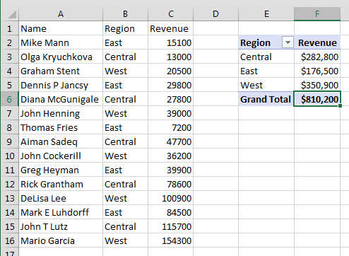
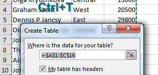
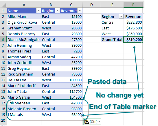
Say that you want to be able to easily add new data below the pivot table, as shown below. Select one cell in the data and press Ctrl+T. Make sure that My Table Has Headers is checked in the Create Table dialog and click OK.


Choose one cell in the table and press Ctrl+T. In the Create Table dialog, ensure the box for My Table Has Headers is checked.

Choose one cell in the table and press Ctrl+T. In the Create Table dialog, ensure the box for My Table Has Headers is checked.

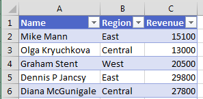
Some nice formatting is applied to the data set. But the formatting is not the important part.

The source data is now formatting in blue.

You have some new records to add to the table. Copy the records.

Three new records (not formatted in blue) have been copied from another worksheet.


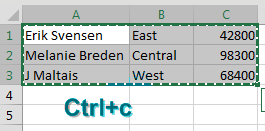
Go to the blank row below the table and paste. The new records pick up the formatting from the table. The angle-bracket-shaped End-of-Table marker moves to C19. But notice that the pivot table has not updated yet.

Paste those three new records in the first row below the source data. The newly pasted records are formatted in blue. The End of Table Marker moves from C16 to C19. (The End of Table Marker is a small right-angle marker in the bottom right corner of the last cell of the table.) Although the new rows are now part of the table, the pivot table has not changed, yet.

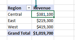
Click the Refresh button in the Pivot Table Tools Analyze tab. Excel adds the new rows to your pivot table.

Choose one cell in the pivot table and click Refresh on the Analyze tab. The numbers change to include the newly pasted data.

Bonus Tip: Use Ctrl+T with VLOOKUP and Charts

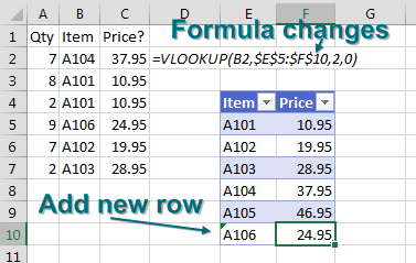
In this figure, the VLOOKUP table is in E5:F9. Item A106 is missing from the table, and the VLOOKUP is returning #N/A. Conventional wisdom says to add A106 to the middle of your VLOOKUP table so you don't have to rewrite the formula.

This screenshot shows a VLOOKUP formula pointing to $E$5:$F$9. Most VLOOKUPs are working, but one item is returning #N/A because that item is missing from the table.

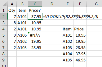
Instead, use Ctrl+T to format the lookup table. Note that the formula is still pointing to E5:F9; nothing changes in the formula.

Before adding the missing item to the lookup table, select one item in the table and press Ctrl+T. Even with the table formatted as a table, the original formula still points to $E$5:$F$9.

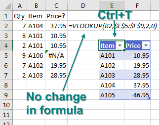
But when you type a new row below the table, it becomes part of the table, and the VLOOKUP formula automatically updates to reflect the new range.

But, miraculously, when you type data in the new row below the lookup table, the VLOOKUP formula automatically rewrites itself to include the new rows.

The same thing happens with charts. The chart on the left is based on A1:B5, which is not a table. Format A1:B5 as a table by pressing Ctrl+T. Add a new row. The row is automatically added to the chart, as shown on the right.

A chart based on Jan, Feb, Mar, Apr data in A2:B5.

Make the chart source data into a table with Ctrl+T. Type new data for May below the original data and the chart automatically updates.

It is fairly cool that you can use Ctrl+T after setting up the pivot table, VLOOKUP, or chart, and Excel still makes the range expand.

When I asked readers to vote for their favorite tips, tables were popular. Thanks to Peter Albert, Snorre Eikeland, Nancy Federice, Colin Michael, James E. Moede, Keyur Patel, and Paul Peton for suggesting this feature. Four readers suggested using OFFSET to create expanding ranges for dynamic charts: Charley Baak, Don Knowles, Francis Logan, and Cecelia Rieb. Tables now do the same thing in most cases.


This article is an excerpt from MrExcel 2024 Igniting Excel

Title photo by Andrei Zolotarev on Unsplash