Excel 2024: Set Up Your Data for Data Analysis

Make sure to follow these rules when you set up your data for sorting, subtotals, filtering and pivot tables.

• Rule 1: Use only a single row of headings above your data. If you need to have a two-row heading, set it up as a single cell with two lines in the row by using Alt+Enter or Word Wrap as discussed in Bonus Tip: Use Accounting Underline to Avoid Tiny Blank Columns.
• Rule 2: Never leave one heading cell blank. This often happens to me when I set up a temporary column.
• Rule 3: There should be no entirely blank rows or blank columns in the middle of your data. It is okay to have an occasional blank cell, but you should have no entirely blank columns.
• Rule 4: If your heading row is not in row 1, be sure to have a blank row between the report title and the headings. It is fine to make this blank row have a row height of 1 so it is barely visible.
• Rule 5: If you have a total row below your data, leave one blank row above the totals.
• Rule 6: Formatting the heading cells in bold will help the Excel's IntelliSense module understand that these are headings.

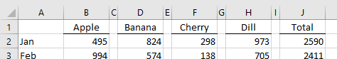
Caution: Following these rules may not help if your data is only two columns wide.

Bonus Tip: Use Accounting Underline to Avoid Tiny Blank Columns

I once worked for a manager who was very particular about the heading underlines in a report.

The manager hated the regular underlines shown in row 1 below. In cell E1, the underline is only as wide as the characters in the cell. If I tried using a bottom border instead of the underline, you would get a single, long, "uniborder" as shown in row 6.

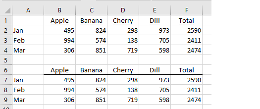
This manager would format his worksheets with tiny little columns between each column. That way, when he used a bottom border, it would go all the way across the cell, but they were still individual borders. This is a data disaster waiting to happen. Someone is going to sort part of the data but not all of the data.

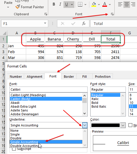
There is an awesome solution, but it is hidden. If you open the Underline drop-down menu on the Home tab of the Ribbon, your only choices are Single or Double. But if you click the dialog launcher in the Font group, the Format Cells dialog offers a drop-down with extra choices for Accounting Underlines. Choose one of those and your underlines will stretch almost all the way across the cell but they will be individual lines instead of a single long line.

---

---

Bonus Tip: Use Alt+Enter to Control Word Wrap

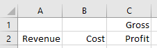
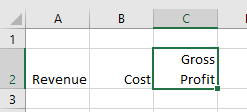
The Gross Profit heading in C1 and C2 violates the rule that each heading should be in a single cell.
In cell C2, type Gross. Then press Alt+Enter. Type Profit. Press Enter. Delete the word Gross from row 1. Excel will see C2 as a single cell. All of the intellisense will continue to work. Why use Alt+Enter instead of turning on Word Wrap? When you have long text that you want to wrap to several lines, the Word Wrap icon frequently wraps at the wrong place.

Alt+Enter prevents this nightmare: in the image below, you type the long heading in D1 and turn on Word Wrap. The results are shown in D3. You don't like where the words are wrapping, so you start typing many spaces at the end of each line as shown in F5. With just the right number of spaces, it will look like D7.

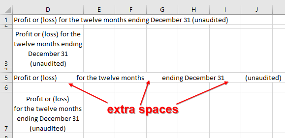
Stop typing all of those spaces. Type the text for line 1, then Alt+Enter.

Bonus Tip: Someone went crazy and used Alt+Enter Too Much

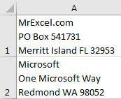
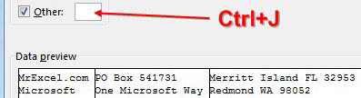
Alt-Enter is a great trick until someone uses it in hundreds of cells. I've seen people treat a single cell as if it were Microsoft Word. Pressing Alt+Enter inserts a Character Code 10 in the cell. You might be tempted to fix this by using =SUBSTITUTE(A1,CHAR(10),","). However, the simple solution is to use Data, Text to Columns. In Step 1, choose Delimited. In Step 2, choose Other. Click into the Other box and press Ctrl+J. You won't see anything in the box, but typing Ctrl+J in this dialog or in the Find & Replace dialog will insert a character 10.