
Excel 2024: Sort and Filter by Color or Icon
April 29, 2024 - by Bill Jelen
Conditional formatting got a lot of new features in Excel 2007, including icon sets and more than three levels of rules. This allows for some pretty interesting formatting over a large range. But once you format the cells, you might want to quickly see all the ones that are formatted a particular way. In Excel 2007, sorting and filtering were also updated to help you do just that!
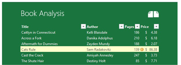
This book analysis table has some highlighted rows to flag interesting books and an icon next to the price if the book is in the top 25% of prices in the list.
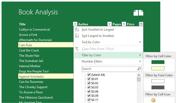
If you want to quickly view all the highlighted rows or cells that have icons, just drop down the filter for the column and choose Filter by Color (or Sort by Color to bubble them to the top).
Then you can pick the formatting you want to sort or filter by! This doesn’t just work for conditional formatting; it also works for manually coloring cells. It is also available on the right-click menu of a cell under the Filter or Sort flyout, and in the Sort dialog.
This tip is from Sam Radakovitz, a project manager on the Excel team. He is more fond of cats than dogs
This article is an excerpt from MrExcel 2024 Igniting Excel
Title photo by Robert Katzki on Unsplash