
Fill Formatting
October 12, 2023 - by Bill Jelen

Problem: I have a thousand rows of data. I want to apply red and blue to every other row. Nothing in the Format as Table looks exactly like I want it to look and I don’t want to define my own table style.
Strategy: This technique temporarily wipes out all of your data, but you get it back. It is a fast way to go.
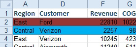
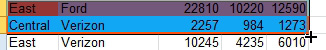
1. Select the data in rows two and three. You will see a fill handle in the bottom right corner of the selection.
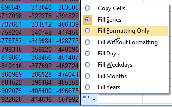
2. Double-click the fill handle. All of your data is destroyed. Don’t panic. Open the icon at the bottom right.
-
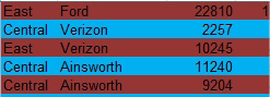
3. Choose Fill Formatting Only. All of your data comes back. The formatting is copied throughout.
Result: the formatting is copied. Your data that was overwritten comes back.
This article is an excerpt from Power Excel With MrExcel
Title photo by Juan Cardenas on Unsplash