
For Each Cell in Column A, Have Three Rows in Column B
September 06, 2023 - by Bill Jelen

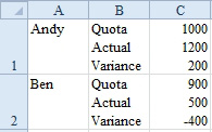
Problem: For each cell in column A, I want to have three rows in columns B and C, as here. I also want to be able to perform calculations with the values in column C.
Strategy: You might be tempted to use the Alt+Enter trick to enter three lines of data in columns B and C. However, this will not work well in column C. Although the numbers are displayed fine, there is no way to have the numbers in C calculate automatically.
A better option is to merge cells A1:A3 into a single cell. You can then let the data in B fill B1:B3. Here’s how:
1. Enter a value in A1. Leave cells A2:A3 blank. Select cells A1:A3.
-
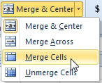
2. Select Home, Merge & Center dropdown. Choose Merge Cells.
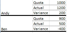
Gotcha: Notice that the vertical alignment defaults to the bottom. This looks okay in a normal-height cell, but not so good in a triple-height cell.
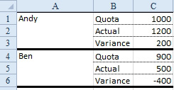
3. Change the vertical alignment to top or center. Vertical alignment icons are now on the Home tab.

4. Creative use of the Borders setting around each group will further enhance the illusion of three rows for each value in column A.
5. If you have several rows that need this formatting, use Format Painter mode to copy the formatting. Select cells A1:A3. Double-click the Format Painter icon in the Home ribbon tab. The double-click will put you in Format Painter mode. You can now click in A4, then A7, then A10. Each click will copy the format from A1:A3 to the clicked cell. When you are finished, you can either click the Format Painter icon or press Esc to exit Format Painter mode.
This article is an excerpt from Power Excel With MrExcel
Title photo by Crissy Jarvis on Unsplash