Function To Merge Two Columns

May 07, 2002 - by Bill Jelen

Cheryl sent in this week's Excel problem. Excel veterans will see this as basic, but it was a valuable tip to Cheryl. Since this is the first Excel tip of the 1999-2000 season, we'll start with a basic one.

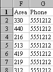
Someone gave me an Excel spreadsheet. Area codes are in column F, and a 7 digit phone number is in column G. I know how to split a column apart using Text-to-Columns, but how do I merge these 2 columns together?

Luckily, area codes and telephone numbers never start with 0 in the U.S., so there were no instances where the leading zero of the phone number was lost. A quick scan of the data showed that all phone numbers had 7 digits and all area codes had three digits. After talking Cheryl, we agreed that the best format would be to have the phone number appear like this: (330) 555-1212

In cell H2, we will start to build the formula. The operator in Excel to join two text fields is the & symbol. Any constants that you want must be included in double quotes. So, to get the leading parentheses and the area code, you need a formula like this: ="("&F2

Next, add another concatenation operator and the closing parentheses around the area code. Note that there is both a parenthese and a space enclosed in the quotes. ="("&F2&") "

To get the phone number with the dash will be a bit more difficult. Use the LEFT function to get just the first three digits of the phone number. The syntax is LEFT(cell,# of characters). After this, add another concatenation character and the middle dash in quotes. ="("&F2&")"&LEFT(G2,3)&"-"

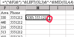
To get the 4th through 7th digits of the phone number, use the MID function. The syntax is MID(cell,Start Character,Number of Characters). We want to start at the 4th character and continue for a total of 4 characters. Thus, the final formula is: ="("&F2&") "&LEFT(G2,3)&"-"&MID(G2,4,4)

Wow - that looks like a big formula, but if you break it down and just build it one step at a time, it is easy.

Follow along for 2 more hot tips. Now that you have the formula in cell H2, you need a fast way to copy it down to all cells. Excel has a great shortcut for this. Put the cellpointer on H2. In the lower right corner of the cellpointer box is a small square. Double click this square with your mouse and the formula will copy down to as many rows as you have data in column G.

There is one last important step. If you would now delete columns F and G, all of those lovely phone numbers in H would turn into #REF!. You need to convert the cells from a formula to values. Here is how to do that. Highlight all of the cells containing phone numbers in column H. Hit Ctrl + C (or Edit - Copy) to copy those cells. Now, without unhighlighting the cells, immediately do an Edit - Paste Special. Click the radio button for Values and click OK. The formulas will now be changed to values and you can delete columns F & G.

Excel is incredibly flexible at manipulating data. In this case, Cheryl was afraid she would be up all night re-keying those area codes and phone numbers into a single cell. The formula and steps in this weeks tip allow you to do the same task in about a minute.