How to See Headings as You Scroll Around a Report

August 27, 2021 - by Bill Jelen

Problem: I have a spreadsheet that has headings at the top. I want to scroll through the data and always see the headings.

There is a big Title in A1, blank row 2, column headings in row 3, and then data starting in row 4. You need to keep row 2 in view as you scroll down. — Figure 61. You want to see row 3 headings even if you scroll to row 800.

Strategy: Select one cell in the data. Press Ctrl+T and click OK. Your data will be formatted. When you scroll the headings out of view, the headings will replace column letters A, B, C.

When formatted as a Ctrl+T table, if you scroll the headings out of view, the column letters A, B, C, and so on are replaced by headings of Rep, Customer, Product, and so on. — Figure 62. Tables will keep the headings in view.

This strategy uses the table concept introduced in Excel 2007. It automatically adds Filter dropdowns and formats the table. It also precludes the use of some features like the View Manager. For a more flexible strategy, use Freeze Panes as discussed next.

Alternate Strategy: You can use the Freeze Panes command on the View tab. In order to make the Freeze Panes command work, you must place the cell pointer in the correct location before using the command.

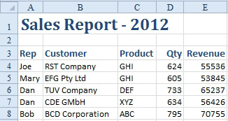
In the spreadsheet shown in Figure 61 it would be really handy to have row 3 always visible while you scroll. Here’s how you make that happen:

1. Use the arrow at the bottom of the vertical scrollbar to move row 3 to the top of the window.
2. Place the cell pointer in cell A4. You’re going to use the Freeze Panes command, which will freeze all visible rows above the cell pointer and all visible columns to the left of the cell pointer. If you place the cell pointer on the heading for column A, you will not freeze any columns, only the rows.

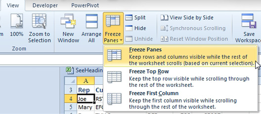
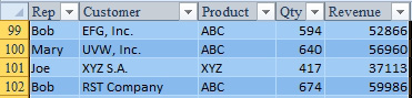
Another great technique requires you to scroll so that the headings in row 3 are at the top of the window. Then, from A4, use Freeze Panes. Everything above the active cell is frozen. — Figure 63. Cells above and left of the active cell is frozen.

3. With the cell pointer in cell A4, select View , Freeze Panes , Freeze Panes. A solid horizontal line will be drawn between rows 3 and 4. As you scroll down, you will always be able to see the heading rows.

Additional Details: To turn off this feature, go to the View tab and select Freeze Panes, Unfreeze Panes. The Unfreeze Panes menu item is visible only after you have frozen the panes.

This article is an excerpt from Power Excel With MrExcel

Title photo by Andres Herrera on Unsplash