Return the Last Entry

May 02, 2022 - by Bill Jelen

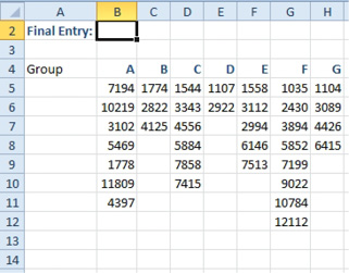
Problem: Someone has logged some data. For each group, data starts in row 5 and continues down for some number of rows. There are a different number of data points in each column. I need to get the last entry in each column.

Strategy: There are multiple solutions to this problem. You could combine the unwieldy OFFSET with COUNT, but this topic will show you how to solve the problem using the approximate match version of VLOOKUP.

Flip back to Figures 390 and 391 where you used the approximate match version of VLOOKUP to find a commission rate. The table had entries like 1000, 5000, 10000, and 20000. When someone had a sale of $12,345, the VLOOKUP would find the commission rate for the $10,000 level, because $10,000 was just less than the $12,345 that you were looking up.

7 columns of data, labeled A through G. Each column has the first number in row 5. But there are a different number of numbers in each column. You want to find the last value in the list. — Figure 444. Return the last number in the column.

In this case, the data is not sorted nor should it be sorted. However, if you ask VLOOKUP to look for a really large number, it will automatically return the last non-blank entry in the column!

Some will suggest that you should use 9.99999999999999E+307 as the lookup value. This is the largest number possible in Excel. However, rather than type all of those characters, you can simply use a number that is larger than anyone would expect. For example, if you work for a company that has $1 Million in revenue per year, there is no way that the sales for one day would ever exceed $100K. You could safely search for 99999.

In the formula below, I held down the 9 key for a second and ended up searching for 9.9 million. It doesn’t matter exactly what you are searching for, just so long as it is larger than any possible number in the list. Use =VLOOKUP(9999999,B5:B20,1,TRUE).

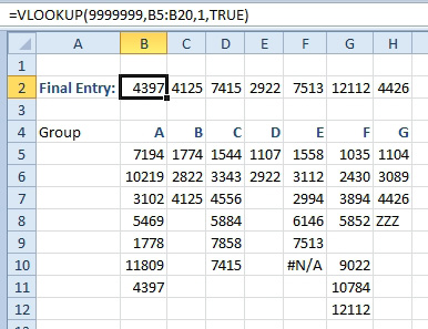
To find the last entry, do a VLOOKUP for a number larger than any possible value. Here =VLOOKUP(9999999. Make sure to put ,TRUE at the end of the VLOOKUP. — Figure 445. This VLOOKUP returns the last numeric value.

This is a really cool use of the rare version of VLOOKUP. As you can see in column G, the formula doesn’t get confused by blank cells. It will only return numeric values, so the errant ZZZ entry in H8 is ignored. The #N/A error in F10 is ignored.

If the entries in the column are text, then you would search for some text which will occur alphabetically after any text that you might expect. For example, search for “ZZZZZZ”.

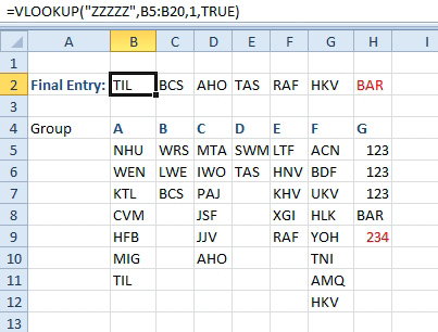
To find the last text entry in each column, do a VLOOKUP for "ZZZZZZZZZ". This will fail if some of the entries are numeric. — Figure 446. Search for ZZZZZZ to return the last text entry.

Column H above illustrates a problem with this method. If the values can contain text or a number, the VLOOKUP will not work.

What if the data is turned sideways and you need to get the last value from each row? Use HLOOKUP instead of VLOOKUP.

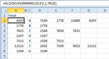
To find the last number in each row, do an HLOOKUP for 9999999 with a ,True at the end of the VLOOKUP. — Figure 447. Get the last entry from each row.

Additional Details: You do not have to put the ,TRUE at the end of any of these formulas. If you leave off the fourth argument, Excel assumes that you mean TRUE. However, since 99.9% of the VLOOKUPs in the world use FALSE at the end, I put the TRUE out there to help remind me that something unusual is happening with this formula.

This article is an excerpt from Power Excel With MrExcel

Title photo by Shwetha Shankar on Unsplash