Return the Last Matching Value

May 03, 2022 - by Bill Jelen

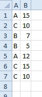
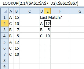
Problem: VLOOKUP returns the first match that it finds. I need to get the last match in the data. In this figure, I want to lookup A and find the 12 from row 5, since that is the latest data for A.

Letters A, C, B, B, A, C, C are in A1:A7. Numbers are in column B. You want to find the match for the last occurence of each letter. — Figure 448. Find the last match for each letter.

Strategy: Use:

=LOOKUP(2,1/($A$1:$A$7=D2),$B$1:$B$7).

Before XLOOKUP, you would have to LOOKUP(2, where the lookup vector is 1/(A1:A7=D2. This formula segment delivers a lot of Division by Zero values and some numbers. By searching for a 2, you are repeating the trick where you are looking for an impossibly large number, and you get the last match. — Figure 449. No one at your office will have a clue what you are doing.

First, LOOKUP is an ancient function that Excel includes for backward compatibility with Quattro Pro. It is a bizarre little function that takes a lookup value, a lookup vector, and a results vector. It always uses the Approximate Match version that you would get when using TRUE at the end of your VLOOKUP. Like the approximate match, LOOKUP expects the table to be sorted, but since you are using this formula to trick Excel, the table does not have to be sorted.

People end up using LOOKUP instead of VLOOKUP because LOOKUP works with arrays that VLOOKUP won’t work with. Both this topic and the next topic show of the array-handling ability of LOOKUP.

This formula came from the MrExcel Message Board, originally posted to a MrExcel MVP named Fairwinds.

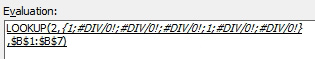
Let me explain the formula step by step, starting with A1:A7=D2. This comparison will produce a series of TRUE/FALSE values. In the figure above, you would end up with {TRUE; FALSE; FALSE; FALSE; TRUE; FALSE; FALSE}.

Next, the formula divides that array into the number 1. Flip back to Figure 387 to see that Excel treats TRUE like 1 and FALSE like 0. Of course, 1/1 is 1. But 1/0 is a DIV/0 error. After doing the division, you have a series of values that are either 1 or #DIV/0!: {1; #DIV/0!; #DIV/0!; #DIV/0!; 1; #DIV/0!; #DIV/0!}.

Evaluate Formula for the LOOKUP function shows you are looking up 2 into an array that says 1, Error, Error, Error, 1, Error, Error. This will find the final 1. — Figure 450. From the Evaluate Formula dialog, after the fourth step.

If you flip back to Figure 445, you can see that the approximate VLOOKUP is ignoring text entries and error values. The same thing works here.

Also, in the last topic, there was a question if you should look for 9.99999999999999E+307 or simply 99999999. As you learned in the last topic, you just have to search for a number that is larger than any expected value. The logical test is either going to return 1 or #DIV/0!. There is no way that you will ever get anything larger than a 1 at this point of the formula. So, you can simply search for a 2.

When LOOKUP is searching for a 2 in {1; #DIV/0!; #DIV/0!; #DIV/0!; 1; #DIV/0!; #DIV/0!}, it can not find the 2. It thus uses the last numeric entry. In this case, it is the 1 that was calculated from cell A5. LOOKUP will return the fifth entry from the results vector. Since the results vector is B1:B7, Excel will return the 12 from cell B5.

Additional Details: The community of Excel aficionados at the MrExcel.com Message Board create some of the wildest formulas that I’ve ever seen. I took a collection of these formulas and put them in my book, Excel Gurus Gone Wild.

This article is an excerpt from Power Excel With MrExcel

Title photo by Nathan Dumlao on Unsplash