Return the Next Larger Value in a Lookup

April 25, 2022 - by Bill Jelen

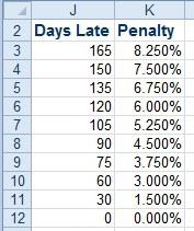
Problem: I am using a lookup table to calculate a late-payment penalty. As soon as a customer is 1 day late, they are charged the penalty for the first month. When they reach 31 days late, they pay for two months. After 60 days late, they are billed for half months.

Strategy: Earlier in “Nest IF Statements”, there was an example using the approximate version of VLOOKUP. This rare version would look for a match. When one is not found, it would return the row just smaller than the lookup value. In this case, you need the VLOOKUP to go the opposite way. VLOOKUP can not do that, but MATCH can.

Make sure that your penalty lookup table is sorted from high to low.

There is a penalty applied depending on how many days late you make your payment. This time, you want to find the next higher penalty bucket. If you are 31 days late, you are paying the penalty associated with 60. — Figure 431. Another rarity: the lookup table sorted descending.

You will see this calculation take shape after many intermediate steps. In real life, you could do all of these steps in a single formula.

Calculate a Penalty Row in F2 with =MATCH(E2,$J$3:$J$12,-1).

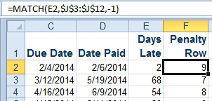
Use the MATCH function with a final argument of -1 to ask for the value just higher than what you are looking up. The lookup table has to be sorted descending. The new XLOOKUP will make this easier. — Figure 432. Find the row with the appropriate penalty.

Take a look at the results of that formula. In row 5, the payment is 30 days late. There is an exact match in Figure 431 for 30 days late, so the formula returns the exact match. However, in rows 2 through 4, there is no exact match. Because the third argument of MATCH is -1, Excel is returning the result from the next higher row in the table. The 68 days late in F3 is matched to the 75-day penalty in row 7 of the table.

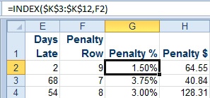
Days Late in E. Penalty Row in F. Then an INDEX in G brings the Penalty Percentage into the grid. — Figure 433. Use INDEX to return the Penalty % from the table.

This is a third example of something that you can do with MATCH and INDEX that you can not do with a regular VLOOKUP.

This article is an excerpt from Power Excel With MrExcel

Title photo by Vanesa Giaconi on Unsplash