
Speed Up Your VLOOKUP
April 22, 2022 - by Bill Jelen

Problem: I have to do thousands of VLOOKUPs and they are taking almost a minute every time that I recalculate the worksheet.
Strategy: Although it is counter-intuitive, two VLOOKUPs with the True argument will run over 100 times faster than the typical VLOOKUP. This is one time the lookup table will have to be sorted.
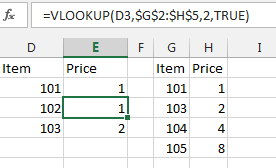
Gotcha: The reason you don’t use the True version of VLOOKUP is that it returns the wrong answer when the key field is not found. In the figure below, item 102 is missing from the lookup table. Instead of returning #N/A, the True version of VLOOKUP returns the answer from the next-lower item number. This is useless and dangerous!
The foremost expert on Formula Speed is Charles Williams, creator of the FastExcelV3 utility. While most people would give up on the True version of VLOOKUP after seeing the above error, Charles realized that the True version of VLOOKUP is hundred times faster than the False version of VLOOKUP.
So, Charles thought up the idea of doing an extra VLOOKUP(A2,Table,1,True) before the real VLOOKUP. When you do a VLOOKUP to return the 1st item in the lookup table, you would normally get back the same value that you are looking up. In other words, =VLOOKUP(101,G2:H5,1,True) better return 101. If it returns something other than 101, then you know that the item is not found.
In the figure below, a formula in column C does a VLOOKUP to return column 1 from the lookup table. A formula in column D checks to see if B2=C2. If the result in D is True, then you know it is safe to do a VLOOKUP in column E. Otherwise, you should report that the value is Not Found.
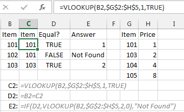
You don’t have to do this in three columns as shown above. You can do a single formula with two VLOOKUPs: =IF(D2=VLOOKUP(D2,$G$2:$H$5,1,TRUE),VLOOKUP(D2, $G$2:$H$5,2,TRUE),”N/A”)
If you see my live seminar, I probably showed how to use FastExcelV3 to time these formulas. I routinely take a 40-second recalc time and have it go to 0.2 seconds by using this formula. It is worth the hassle if you have a spreadsheet that is taking forever to calculate.
Note: This page contains just 1 of hundreds of amazing tricks from Charles Williams. Check out FastExcelV3.
This article is an excerpt from Power Excel With MrExcel