
Summarize Pivot Table Data by Three Measures
November 22, 2022 - by Bill Jelen

Problem: I want to summarize data by region, product, and customer. How can I use a two-dimensional report to show three dimensions of data?
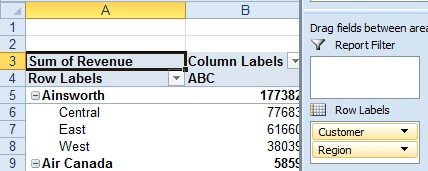
Strategy: Several views of the data are possible. Say that you are starting with products across the top and customers down the side. From the top of the PivotTable Field List dialog, you click the Region field. It is automatically added as the last row field. The view below shows the first customer and the purchases by region.
Another option is to drag the Region field heading above the Customer field heading in the bottom of the Field List dialog. Watch for the blue insertion bar.
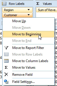
If your mouse is not accurate enough to complete this drop, you can move the Product field to the Row Labels drop zone. Then you open the dropdown arrow at the right side of the Product field in the bottom of the Field List dialog and choose Move Up or Move to Beginning.
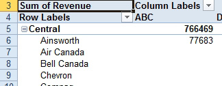
Results: By changing the order of the fields in the row area, you now see the first region and all of the customers in that region.
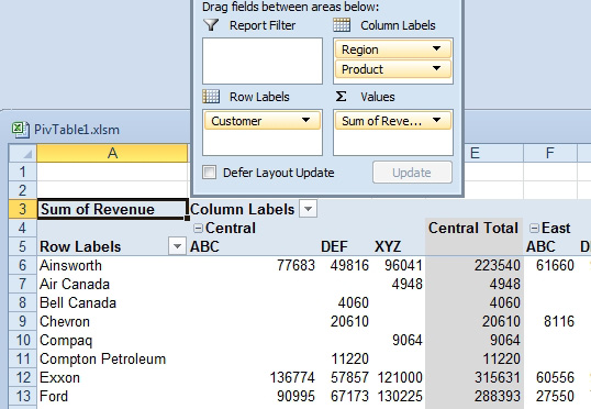
You can also stack fields in the Column Labels drop zone.
This article is an excerpt from Power Excel With MrExcel