
Top Five Report
August 08, 2017 - by Bill Jelen

The pivot table Top 10 Filter gives a total of the visible rows
Pivot tables offer a Top 10 filter. It is cool. It is flexible. But I hate it, and I will tell you why.
Here is a pivot table showing revenue by customer. The revenue total is $6.7 million.
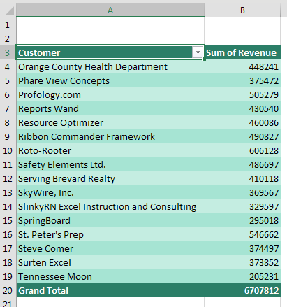
What if my manager has the attention span of a goldfish and wants to see only the top five customers?
To start, open the dropdown in A3 and select Value Filters, Top 10.
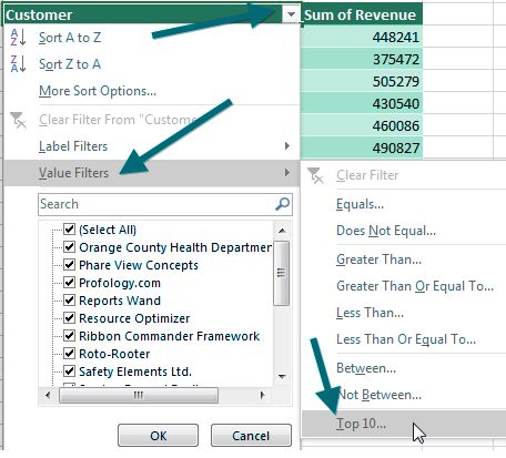
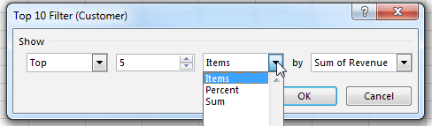
The super-flexible Top 10 Filter dialog allows Top/Bottom. It can do 10, 5, or any other number. You can ask for the top five items, top 80%, or enough customers to get to $5 million.
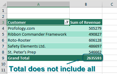
But here is the problem: The resulting report shows five customers and the total from those customers instead of the totals from everyone.
But First, a Few Important Words About AutoFilter
I realize this seems like an off-the-wall question. If you want to turn on the Filter dropdowns on a regular data set, how do you do it? Here are three really common ways:
- Select one cell in your data and click the Filter icon on the Data tab.
- Select all of your data with Ctrl + * and click the Filter icon on the Data tab.
- Press Ctrl + T to format the data as a table.
These are three really good ways. As long as you know any of them, there is absolutely no need to know another way. But here's an incredibly obscure but magical way to turn on the filter:
- Go to your row of headers, go to the rightmost heading cell. Move one cell to the right. For some unknown reason, when you are in this cell and click the Filter icon, Excel filters the data set to your left. I have no idea why this works. It really isn’t worth talking about because there are already three really good ways to turn on the Filter dropdowns. I call this cell the Magic cell.
And now, Back to Pivot Tables...
So, there is a rule that says you cannot use the AutoFilters when you are in a pivot table. See below? The Filter icon is grayed out because I’ve selected a cell in the pivot table.
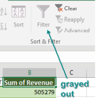
I never really considered why Microsoft grays this out. It must be something internal that says AutoFilter and a Pivot Table can’t coexist. So, there is someone on the Excel team who is in charge of graying out the Filter icon. That person has never heard of the Magic cell. Select a cell in the pivot table, and the Filter gets grayed out. Click outside of the pivot table, and Filter is enabled again.
But wait. What about the Magic cell I just told you about? If you click in the cell to the right of the last heading, Excel forgets to gray out the Filter icon!
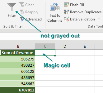

Sure enough, Excel adds AutoFilter dropdowns to the top row of your pivot table. And the AutoFilter operates differently than pivot table filters. Go to the Revenue dropdown and choose Number Filters, Top 10...
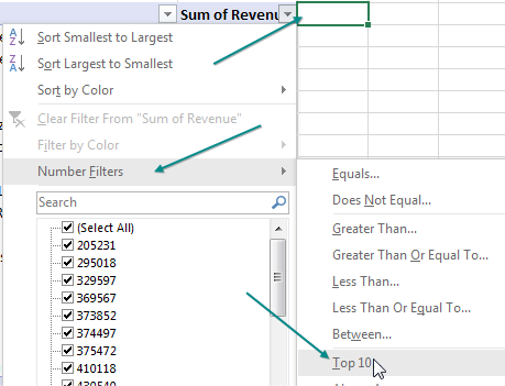
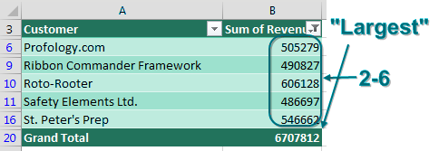
In the Top 10 AutoFilter dialog, choose Top 6 Items. That’s not a typo…. If you want five customers, choose 6. If you want 10 customers, choose 11.
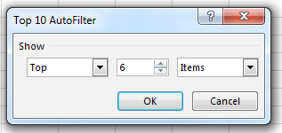
To AutoFilter, the grand total row is the largest item in the data. The top five customers are occupying positions 2 through 6 in the data.
Caution
Clearly, you are tearing a hole in the fabric of Excel with this trick. If you later change the underlying data and refresh your pivot table, Excel will not refresh the filter, because, as far as Microsoft knows, there is no way to apply a filter to a pivot table!
Note
Our goal is to keep this a secret from Microsoft, because it is a pretty cool feature. It has been “broken” for quite some time, so there are a lot of people who might be relying on it by now.
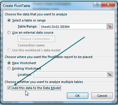
If you want a pivot table showing you the top five customers but the total from all customers, you have to move your data outside of Excel. If you have Excel 2013 or 2016, there is a very convenient way to do this. To show you this, I’ve deleted the original pivot table. Choose Insert, Pivot Table. Before clicking OK, select the box that says Add This Data to the Data Model.
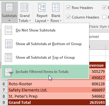
Build your pivot table as normal. Use the dropdown in A3 to select Value Filters, Top 10, and ask for the top five customers. With one cell in the pivot table selected, go to the Design tab in the ribbon and open the Subtotals dropdown. The final choice in the dropdown is Include Filtered Items in Totals. Normally, this choice is grayed out. But because the data is stored in the Data Model instead of a normal pivot cache, this option is now available.
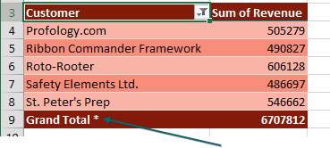
Choose the Include Filtered Items in Total option, and your Grand Total now includes an asterisk and the total of all of the data.
This trick originally came to me from Dan in my seminar in Philadelphia. Thanks to Miguel Caballero for suggesting this feature.
Watch Video
- The pivot table Top 10 Filter gives a total of the visible rows
- Include Filtered Items in Totals is Greyed Out
- Odd way to invoke the Data Filter from the magic cell
- Data Filters are not allowed in pivot tables
- Excel fails to grey out the Data Filter from the magic cell
- Ask for the top 6 to get top 5 plus Grand Total
- Useful for filtering by a specific pivot item
- Excel 2013 or newer: Different Way to get the True Total
- Send your data through the Data Model
- Include Filtered Items in Totals will be available
- Get Total with asterisk
- I learned this trick 10+ years ago from Dan in Philadelphia
Video Transcript
Learn Excel for MrExcel Podcast, Episode 1999 -- Pivot Table True Top Five
I am podcasting this entire book. There's a playlist, click the I on the top right hand corner to follow that playlist. Welcome back to the MrExcel netcast. I'm Bill Jelen.
Alright, so we're going to create a Pivot Table and we want to show, not all the customers, but just the top five customers. INSERT, Pivot Table. Okay, I'll put Customer down the left-hand side and Revenue. Alright so here's our whole list of customers noted as 6.7 million dollars. Excel, makes it easy to do a top five. Go into Row Labels, Value Filters, top 10. Doesn't have to be top. It can be top or bottom. Doesn't have to be five. It can be twenty, forty, it can be whatever. Top eighty percent, give me enough records to get to three million dollars or four million dollars, but here we go. Top five items. Now remember 6.7 million dollars, click OK and my big problem here, is that, that grand total is not the 6.7 million. When I give this to the VP of sales he's going to freak out, saying, wait a second, I know I did more than 3.3 million dollars. Right, so we're going to undo, undo that and go back to the original data.
Now this next trick I learned during one of my Power Excel Seminars in Philadelphia. A guy named Dan in row two, showed me this. It was more than ten years ago that he showed me this trick, and first we have to talk about the Filters. So normally, if you're going to use the regular Filter, this Filter here, you choose any one cell in your data set and click the Filter Icon, or some people choose the whole Data Set, CONTROL* and click the Filter Icon, but there's a third way. A way that nobody cares about. If you go to the very last Heading Cell, in my case, that's Cost in L1, and go one cell to the right. I call this the magic cell, I have no idea why but for some unknown reason, from this cell, I can filter the adjacent Data Set. Alright, it's like a weird way and no one cares about this.
Right, because there's two other really good ways to invoke a Filter, no one needs to know about the magic cell, but here's the thing, see inside of a Pivot Table, it's grayed out. You're not allowed to use those Filters. It's against the rules. Now, if I come out here, I'm more than welcome to use the Filter but inside they grade out. I don't know who the person is who grays this out, but they've never heard my little talk about the magic cell, because if I go to the very last Heading Cell and go one cell to the right, look at that, they forget to grey out the Filter and now I've just added the old Auto Filters to the Pivot Table. So I come here, go to Number Filters, that's different than Value Filters. It's still called Top Ten. Slightly different, I'm going to ask for the top five, no the top six. The top six because to this Filter the Grand Total is just another row, and the Grand Total is the largest item and then when asked for items 2 through 6, I get the top five items.
Alright, so there we are. A cool Filter hack, that gives us the top five items and the true total of everybody. Alright now, a couple things. Don't forget about the magic cell. Alright there's no way to turn this Filter off, unless you go back to the magic cell. Alright so you need to remember the magic cell. Also, if you change the underlying data and you refresh the Pivot Table, they're not going to refresh the Filter because as far as Microsoft knows, you're not allowed to have a Filter.
This is useful for other things. Sometimes we have products going across the top. Let's go here at a tabular form. Not necessary, I just like to get real headings. Gizmo, Widget, Gadgets, Doodads. Alright and maybe you're the manager of Doodads and you need to see just the customers who had a particular value and Doodads. So I go to the magic cell, turn on the Filter and then under Doodads I can ask for items that are greater than zero. Click OK. Alright, that type type of Filtering would not be possible on a regular Pivot Table, but it is possible using the magic cell.
Alright now let's undo the list. Let's turn off this Filter and remove the Pivot Table, and if you're in Excel 2013 or new, I'm going to show you a completely legal way to get the correct total at the bottom. Insert Pivot Table, down here at the bottom, starting in Excel 2013 this very innocuous box, doesn't sound very exciting, add this data to the Data Model. That sends the data, behind the scenes, to the Power Pivot Engine. Build the exact same report. Customers down the left-hand side. Revenue in the heart of the Pivot Table. Then, go to the regular Filters, the Value Filters top 10. Ask for the top five. Notice again we have 6.7 million dollars after I do this, 3.3 million dollars but here's the difference. When I go to the Design Tab, under Subtotals, this feature called Include Filtered Items in Totals, is no longer grayed out. At a regular Pivot Table is not available. We get a little asterisk there and it's the total of everything. Alright, now of course that only works in Excel 2013 or newer.
Alright it's going to take six weeks for me to get this entire book out here on YouTube. There's so many good tips here. Tips that could start to save you time, right away. Buy the entire book right now and you'll have access to all 40, It's actually a lot more than 40 tips. Excel shortcut keys. All kinds of great stuff in this book.
Alright, recap. So when we do a Pivot Table top 10 Filter, it gives us the total but only the visible rows, not the stuff that it filtered out. Yeah if we go to the second tab and look for Subtotals, Filtered Items and Totals, it's grayed out, but there is an odd way to invoke the Old Data Filter from the magic cell. The very last heading cell, go one cell to the right, you can't use Filters and Pivot Tables, but if you go to the magic cell they forget to gray it out. Now in the Number Filter, you ask for the top six to get the top five, plus the grand total. Also useful for filtering to a specific Pivot Item: Doodads, anything that had greater than 0 in Doodads or top 5 Doodads. Excel 2013 or newer, there's a different way to get the True Total. Check that box for the Data Model and then include Filtered Items in Totals will be available. You get the total with an asterisk. And thanks to Dan in Philadelphia who showed me at one of my Power Excel Seminars, more than ten years ago, and gave me this great little trick. A way for the Filter to sneak through the Club Pivot Table Wall. They normally don't allow that Auto Filter.
Hey, I want to thank you for stopping by. We'll see you next time, for another netcast from MRExcel.
Download File
Download the sample file here: Podcast1999.xlsx
Title Photo: Gadini / pixabay