Total the Red Cells

January 10, 2022 - by Bill Jelen

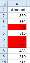
Problem: I’ve marked several cells in red. I need to total the red cells.

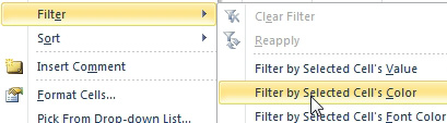
The heading in A1 says Amount. Several numbers are shown, with three cells having a red fill. What is the total of the red numbers? — Figure 265. Total the red cells.

Strategy: Use the new filter by color to show only the red cells. Right-click on a red cell and choose Filter, Filter by Cell Color.

Right-click one red cell, choose Filter, then Fill by Selected Cell's Color. — Figure 266. Choose to filter by cell color.

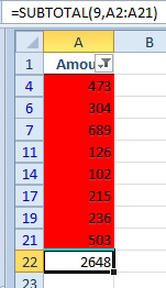
Only the red cells will be shown. After applying the filter, go to the first visible blank cell below the data and press the AutoSum button or Alt+Equals. When applied to a filtered dataset, the AutoSum button switches from the SUM function to the SUBTOTAL function. This function will sum only the visible cells, providing a sum of the red cells.

Only the heading and the red cells are shown: A4, A6, A7, A11, A14, A17, A19, and A21. From the blank cell in A22, press the AutoSum. Excel writes a formula =SUBTOTAL(9,A2:A21) which totals only the visible cells. The total is 2648. — Figure 267. AutoSum uses SUBTOTAL now.

Additional Details: This feature will work even if the red has been applied by conditional formatting.

Gotcha: When you clear the filter to show all cells, the formula will include the non-red cells. If you need a formula to add the red cells while displaying the other cells, you would have to use a User Defined Function in the Excel VBA language. Watch this YouTube video: https://mrx.cl/sumredmacro for details.

This article is an excerpt from Power Excel With MrExcel

Title photo by Ed Leszczynskl on Unsplash