
UNIQUE From Non-Adjacent Columns
November 15, 2018 - by Bill Jelen

The other day, I was about to create a unique combination of two non-adjacent columns in Excel. I usually do this with Remove Duplicates or with Advanced Filter, but I thought I would try to do it with the new UNIQUE function coming to Office 365 in 2019. I tried several ideas and none would work. So, I went to the master of Dynamic Arrays, Joe McDaid, for assistance. The answer is pretty cool, and I am sure I will forget it, so I am documenting it for you and for me. I am sure, two years from now, I will Google how to do this and realize "Oh, look! I am the one who wrote the article about this!"
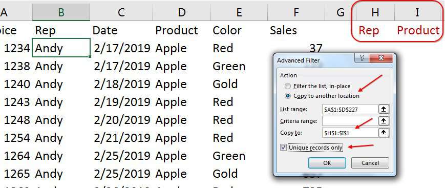
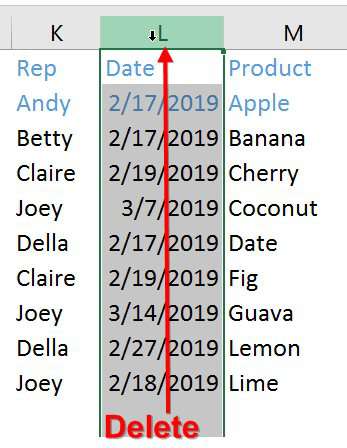
Before getting to the UNIQUE function, take a look at what I am trying to do. I want every unique combination of Sales Rep from column B and Product from column C. Normally, I would follow these steps:
- Copy the headings from B1 and D1 to a blank section of the worksheet
- From B1, choose Data, Filter, Advanced
- In the Advanced Filter dialog, choose Copy To A New Location
- Specify the headings from Step 1 as the Output range
- Choose the box for Unique Values Only
- Click OK
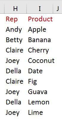
The result is every unique combination of the two fields. Note that the Advanced Filter does not sort the items - they appear in the original sequence.
This process became easier in Excel 2010 thanks to the Remove Duplicates command on the Data tab of the Ribbon. Follow these steps:
- Select B1:D227 and Ctrl + C to Copy
-
Paste to a blank section of the worksheet.
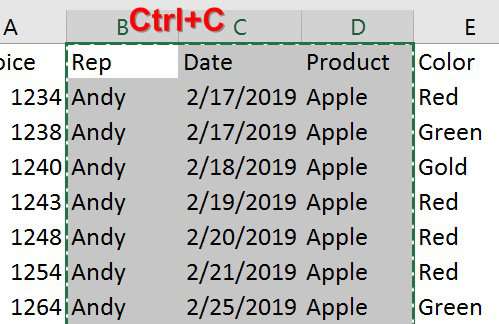
Make a copy of the data since Remove Duplicates is destructive - Choose Data, Remove Duplicates
- In the Remove Duplicates dialog box, unselect Date. This tells Excel to only look at Rep and Product.
-
Click OK
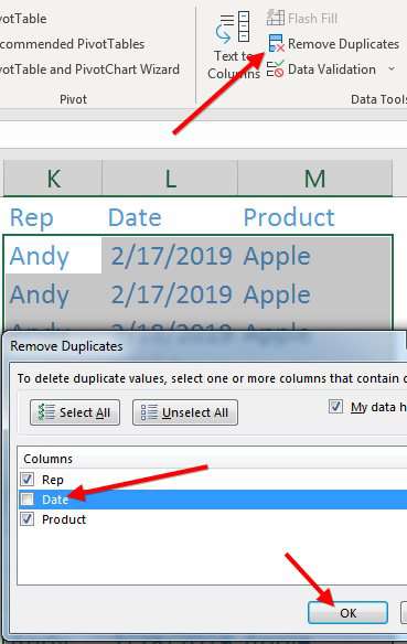
Tell Remove Duplicates to only consider Rep and Date
The results are nearly perfect - you just have to delete the Date column.
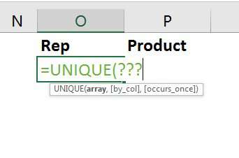
The question: Is there some way to have the UNIQUE function look at only columns B & D? (If you have not seen the new UNIQUE function yet, read: UNIQUE function in Excel.)
Asking for =UNIQUE(B2:D227) would get you every unique combination of Rep, Date, and Product which is not what we are looking for.
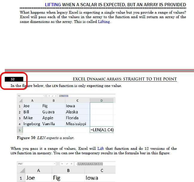
When Dynamic Arrays were introduced in September, I said we would never have to worry about the complexities of Ctrl + Shift + Enter formulas anymore. But to solve this problem, you are going to use a concept called Lifting. Hopefully by now, you've downloaded my Excel Dynamic Arrays Straight To The Point e-book. Turn to pages 31-33 for a complete explanation of Lifting.
Take an Excel function that is expecting a single value. For example, =CHOOSE(Z1,"Apple","Banana") would return either Apple or Banana depending on if Z1 contains 1 (for Apple) or 2 (for Banana). The CHOOSE function is expecting a scalar as the first argument.
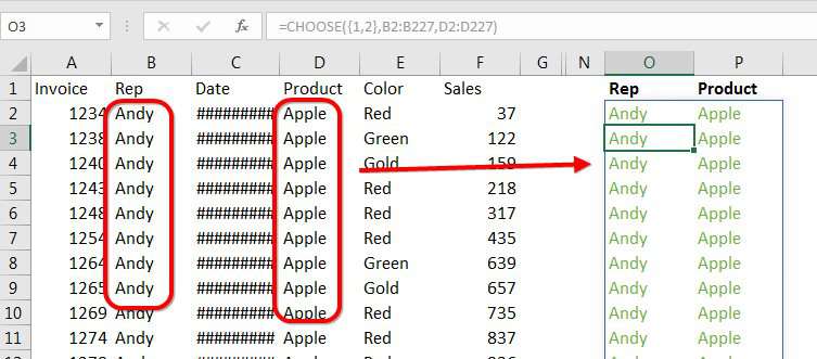
But instead, you are going to pass an array constant of {1,2} as the first argument to CHOOSE. Excel will perform the Lifting operation and calculate CHOOSE twice. For the value of 1, you want the sales reps in B2:B227. For the value of 2, you want the products in D2:D227.
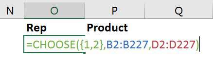
Normally, in old Excel, implicit intersection would have screwed up the results. But now that Excel can spill results to many cells, the formula above successfully returns an array of all answers in B and D:
I feel like I would be insulting your intelligence to write the rest of the article, because from here it is super-simple.
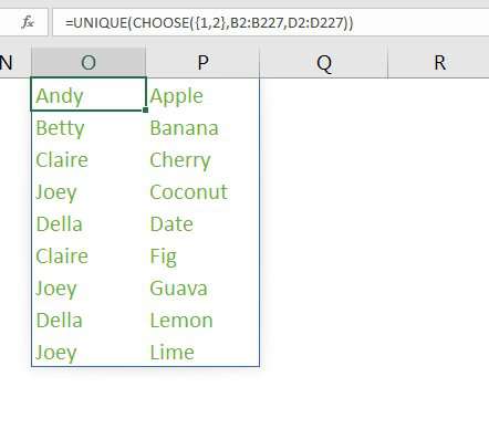
Wrap the formula from the previous screenshot in UNIQUE and you get just the unique combinations of Sales Rep and Product using =UNIQUE(CHOOSE({1,2},B2:B227,D2:D227)).
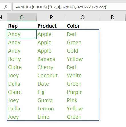
To check your understanding, try to change the above formula to return all unique combinations of three columns: Sales Rep, Product, Color.
First, change the array constant to refer to {1,2,3}.
Then, add a fourth argument to CHOOSE to return color from E2:E227: =UNIQUE(CHOOSE({1,2,3},B2:B227,D2:D227,E2:E227)).
It would be nice to sort those results, so we turn to Sort with a formula using SORT and SORTBY.
Normally, the function to sort by the first column ascending would be =SORT(Array) or =SORT(Array,1,1).
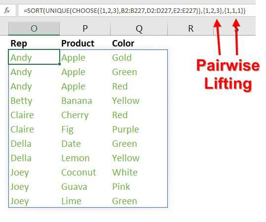
In order to sort by three columns, you need to do some pairwise lifting with =SORT(Array,{1,2,3},{1,1,1}). In this formula, when you get to the second argument of SORT, Excel wants to know by which column to sort. Instead of a single value, send three columns inside an array constant: {1,2,3}. When you get to the third argument where specify 1 for Ascending or -1 for Descending, send an array constant with three 1's to indicate Ascending, Ascending, Ascending. The following screenshot shows =SORT(UNIQUE(CHOOSE({1,2,3},B2:B227,D2:D227,E2:E227)),{1,2,3},{1,1,1}).
At least until the end of 2018, you can download the Excel Dynamic Arrays book for free using the link at the bottom of this page.
I am encouraged to find that the answer to today's question is a bit complicated. When Dynamic Arrays came out, I instantly thought of all of the amazing formulas posted at the MrExcel Message Board by Aladin Akyurek and others and how those formulas would become far simpler in the new Excel. But today's example shows that there will still be a need for formula geniuses to craft new ways to use the Dynamic Arrays.
Watch Video
Download Excel File
To download the excel file: unique-from-non-adjacent-columns.xlsx
Excel Thought Of the Day
I've asked my Excel Master friends for their advice about Excel. Today's thought to ponder:
"Rules for lists: no blank rows, no blank columns, one cell headers, like with like"
Title Photo: The Roaming Platypus on Unsplash