
Use Two-way Interpolation With A Single Formula
April 02, 2021 - by Bill Jelen

Challenge: Many engineering design problems require designers to use tables to compute values of design parameters. Such tables contain values of the required parameter for a range of values of a control parameter, arranged in discrete intervals, and the designer is permitted to use linear interpolation for obtaining the parameter value for intermediate values of the control parameter.
| Height | Velocity |
|---|---|
| 20 | 10 |
| 30 | 40 |
| 40 | 130 |
| 50 | 180 |
| 60 | 240 |
A simple example is a two-column table comprising height above ground (the control parameter) and wind velocity (a design parameter to be read from the table). In the table above, if you need to find the velocity corresponding to a height of 47 meters, it is a fairly simple matter to devise a formula that computes 130 + (180 – 130) * 7 / 10 = 165 meters/sec.
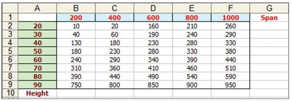
How would you do this for a two-way table in which there are two control parameters? Is it possible to do so using a single formula? The table in Figure 63 illustrates values of wind pressure for the control parameters Height of structure and Span, and you need to compute the wind pressure for a height of 25 meters and a span of 300 meters.
Solution: The procedure you use to solve this problem is essentially an extension of the method used for the single control parameter table. Follow these steps:
- Start with the worksheet shown in Figure 63. Add input cells for height and span in J1 and J2 respectively.
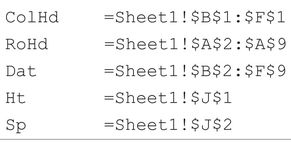
- For ease of formula readability, define the following names:

You can solve the problem using a series of formulas as shown in J3:J17 of Figure 64:
- The MATCH in J3 finds the row number in Figure 63 that is less than or equal to the height in cell J1.
- The MATCH in J5 finds the column number in Figure 63 that is less than or equal to the span in J2.
- Formulas in J4 and J6 add one to the previous cell.
- Formulas in J7:J10 use INDEX functions based on rows J3 & J4 and columns J5 & J6 to get the lower & higher height & spans.
- The HtDiff in J11 is the amount at which the sought height is in excess of the previous height.
- The SpanDiff in J12 is the amount at which the sought span is in excess of the previous span.
- The intervals in J13:J14 calculate the delta between the previous and next height or span.
- Cells J15:J17 then complete the interpolation
Building the Mega-formula
You can now integrate the formulas in J3:J17 into a single formula to get the required wind pressure:
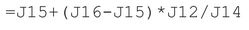
- Copy the text of the formula in J17 to, say, J20—so the formula in J20 is:
- Substitute the cell references for each precedent cell in this formula with the formula in the cell. To illustrate, the first cell reference is J15, which occurs at two places in the formula:

The formula in cell J15 is:
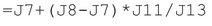
- Copy the text of the formula (without the = sign) and replace the J15s in the formula in J20 so that the formula now becomes:

- Do the same with the remaining references J16, J12, and J14.
- Successively repeat the procedure of back-substitution for the new set of references until all references in the formula are reduced to the defined names ColHd, RoHd, Dat, Ht, and Sp.
The resulting formula, after all substitutions, is:
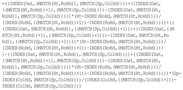
This impressive-looking formula is 867 characters long and, of course, totally incomprehensible in its final form.
Summary: You can build a single formula from a multiple-step calculation, using successive back-substitution, starting with the last formula.
Title Photo: Justin Luebke on Unsplash
This article is an excerpt from Excel Gurus Gone Wild.