Using FILTER with Multiple Conditions

August 17, 2022 - by Bill Jelen

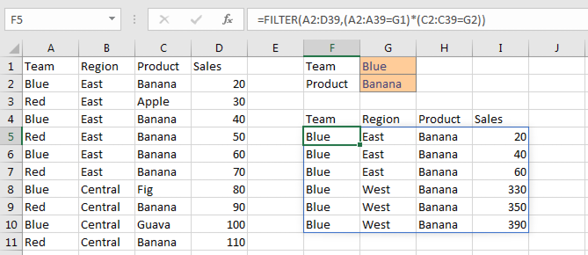
Say you have to combine two criteria, and both criteria have to be true. Wrap each item in parentheses and multiply them together. In the figure below, the formula is =FILTER(A2:D39,(A2:A39=G1)*(C2:C39=G2)). Thanks to Smitty Smith for this technique.

In order to filter to Team=Blue and Product=Banana, you can multiply the conditions: =FILTER(A2:D39,(A2:A39=G1)*(C2:C39=G2)). In this case G1 says Blue and G2 says Banana.

Figure 622. Multiply two sets of conditions to join with

If you want to see all records that are either Fig or Guava, join the conditions with a plus sign:
=FILTER(A2:D39,(C2:C39="Fig")+(C2:C39="Guava"))

For all team Blue records with Fig or Guava:
=FILTER(A2:D39,((C2:C39="Fig")+(C2:C39="Guava"))*(A2:A39=G1))

This article is an excerpt from Power Excel With MrExcel

Title photo by Amy Shamblen on Unsplash