VLOOKUP Left problem

April 20, 2022 - by Bill Jelen

Problem: The lookup table is maintained by another department. They built it with the price to the left of the item number. Can I specify -1 as the third term of the VLOOKUP to indicate that I want a value to the left of the key field?

In this lookup table, the Price is to the left of the part number. VLOOKUP can not easily solve this. — Figure 424. Lookup a value to the left of SKU.

Strategy: Unfortunately, the Excel team doesn’t offer the ability to VLOOKUP to the left of the key field. However, you can use MATCH to figure out which price to use.

Before you see how to solve this with MATCH and INDEX, the obvious solution would be to copy column G over to column J and then do a VLOOKUP. You are suspending reality here and assuming that you can’t move the price. Perhaps the data is coming in from a web query and is refreshed every five minutes?

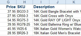
The SKU’s are in H2:H29. They are not sorted, nor do they have to be. Each SKU occurs only once.

Look at the formula in C6. It is =MATCH(A6,$H$2:$H$29,0) which tells Excel to find CR-50 in the range of H2:H29. The final 0 indicates that you are looking for an exact match.

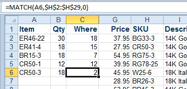
To lookup the price, the first step is to use MATCH to find where the part number is found. — Figure 425. MATCH locates CR50-3 in the lookup table.

Look at the answer from the MATCH function. It says CR50-3 is in row 2, but you can see that CR50-3 is actually in H3 which is row 3 of the spreadsheet. This is an important distinction. MATCH returns the relative position of the item within the lookup range. The answer of 2 says that CR50-3 is in the second cell of H2:H29.

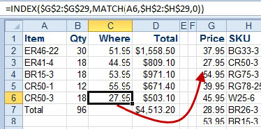
Now that you know the position of the item within the lookup table, you can use the INDEX function to return the price.

You will specify the range of prices as the first argument of the INDEX function. The second argument specifies the row within the lookup table. When you have a single-column lookup table, you do not have to specify the column in the third argument. MATCH assumes you want column 1.

The prices are in G2:G29. Use: =INDEX(G2:G29,MATCH(A6,$H$2:$H$29,0))

Pass the results of the MATCH function to the INDEX function. Index is pointing at the range of prices and returns the price matching the item number. — Figure 426. Essentially a VLOOKUP Left.

This article is an excerpt from Power Excel With MrExcel

Title photo by 愚木混株 cdd20 on Unsplash