Count num. of customers with sales grand total >=100

[Zaoka]

Hi,

Can you help me with the creation of custom measurement that would count number of customers that have Grand total sales greater than 100$

I created this measurement, that count active customers per Sales person and brand if net sales per brand is greater that 0

=COUNTROWS(FILTER(ADDCOLUMNS(SUMMARIZE(SalesSource;SalesSource[DSDBC]);"zaoka";MAXX(VALUES(SalesSource[Brand]);CALCULATE(SUM([Net sales value $]);ALL(SalesSource[Net sales value $]))));[zaoka]>0))

but i don't know how to add code that would first check sales grand total per customer and if sales is >=100$ then count that customer as active per brand.

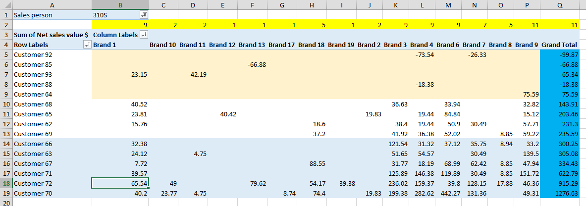
This is Example of data

https://www.dropbox.com/s/79dh21slo42c1hi/Count%20example.xlsb?dl=0

 

[VBA Geek]

Get the file:

https://1drv.ms/x/s!AiiWkkwHZChHjw3tCeHdfpQ4qKkc

 

[Zaoka]

Thank you, but it does not work as i imagined it.


let's put it this way


First condition for customer to be counted is to be over 100 in total sales, second condition is for sales per brand to be over 0 .

(on the above dropbox link I set an example where the first condition is 300 for better understanding, sheet manual check).

 

[VBA Geek]

Using the same measure, if I change the layout of my pivot table:

I tie to your 'manual check' tab:

 

[Zaoka]

Yes, but i already have "Yellow" numbers with custom DAX measurement, i need blue ones

​

https://imgur.com/69JPcIV

(I did re-upload excel example,after your first post sorry for that)

 

[VBA Geek]

Which ones are the blue ones? The value inside the pivot table are just the sum of ''Net sales value $' ?

 

[Zaoka]

(I did re-upload excel example,after your first post sorry for that)
same link in first post

 

[VBA Geek]

Ok, try using this one:

=<br><span class="Keyword" style="color:#0070FF">CALCULATE</span><span class="Parenthesis" style="color:#969696"> (</span><br><span class="indent4">    </span><span class="Keyword" style="color:#0070FF">COUNTROWS</span><span class="Parenthesis" style="color:#969696"> (</span> Customers <span class="Parenthesis" style="color:#969696">)</span>,<br><span class="indent4">    </span><span class="Keyword" style="color:#0070FF">FILTER</span><span class="Parenthesis" style="color:#969696"> (</span><br><span class="indent8">        </span><span class="Keyword" style="color:#0070FF">VALUES</span><span class="Parenthesis" style="color:#969696"> (</span> Customers[Customer code] <span class="Parenthesis" style="color:#969696">)</span>,<br><span class="indent8">        </span><span class="Keyword" style="color:#0070FF">CALCULATE</span><span class="Parenthesis" style="color:#969696"> (</span><br><span class="indent8">        </span><span class="indent4">    </span><span class="Keyword" style="color:#0070FF">SUM</span><span class="Parenthesis" style="color:#969696"> (</span> Sales[Net sales value $] <span class="Parenthesis" style="color:#969696">)</span>,<br><span class="indent8">        </span><span class="indent4">    </span><span class="Keyword" style="color:#0070FF">ALL</span><span class="Parenthesis" style="color:#969696"> (</span> Products[Brand] <span class="Parenthesis" style="color:#969696">)</span><br><span class="indent8">        </span><span class="Parenthesis" style="color:#969696">)</span> >= <span class="Number" style="color:#EE7F18">300</span><br>            && <span class="Keyword" style="color:#0070FF">CALCULATE</span><span class="Parenthesis" style="color:#969696"> (</span><br><span class="indent8">        </span><span class="indent8">        </span><span class="Keyword" style="color:#0070FF">SUM</span><span class="Parenthesis" style="color:#969696"> (</span> Sales[Net sales value $] <span class="Parenthesis" style="color:#969696">)</span><br><span class="indent8">        </span><span class="indent4">    </span><span class="Parenthesis" style="color:#969696">)</span> > <span class="Number" style="color:#EE7F18">0</span><br><span class="indent4">    </span><span class="Parenthesis" style="color:#969696">)</span><br><span class="Parenthesis" style="color:#969696">)</span><br>

 

[Zaoka]

this one work thank you sir, i think i understand,

is it possible to do this without these 2 extra tables?

 

[VBA Geek]

You could but I strongly advise to normalize your data into the 2 dimension tables and one fact table as this is how Power Pivot is supposed to perform best