
Data Visualizations in Excel 2007
November 01, 2007
Excel 2007 offers amazing new data visualization tools such as icon sets, data bars, and color scales. These are great for the manager who's eyes glaze over when presented with a table of numbers.
- Data bars are tiny cell-sized bar charts that can be applied to a range of numbers.
- Color scales allow you to apply a gradient to a range of numbers; think largest numbers in green, smallest numbers in red
- Icon sets allow you to apply traffic light icons to a range of numbers.
To apply a color scale, select a range then choose, Home, Conditional Formatting, Color Scales, and a color scheme. The 4 choices in the top row are three color schemes and work best when displayed in color. The four choices on the bottom are 2-color schemes and work better when printing.

For an icon set, select a range of numbers then choose Home, Conditional Formatting, Icon Sets. The 17 built-in schemes offer a variety of 3, 4, and 5 icon sets. Some of them are only good if you print in color. (For example, the red, yellow, green traffic light will not look good on a black-and-white printout. This icon set offers different shapes (checkmark, exclamation, x) in different colors and looks good whether you are printing or displaying the worksheet.

Data bars provide an in-cell bar chart for each cell. The largest numbers get the largest swath of color and the smaller numbers get a smaller swatch of color. Choose Home, Conditional Formatting, Color Bars, and a color.

Note
For any visualization, choose More from the flyout menu and you can define your own custom colors.
Showing Only Checkmarks
In the segment, I show how to create an icon set where only the top icon is shown. Follow these steps:
- Apply an icon set as usual. All three icons will appear. Note the smallest number with a green checkmark.
-
Use Home, Conditional Formatting, New Rule. Choose Format Only Cells that Contain. In the bottom, choose Cell Value, Less Than, and the number just below the lowest green checkmark. Don't apply any formatting in this rule!

-
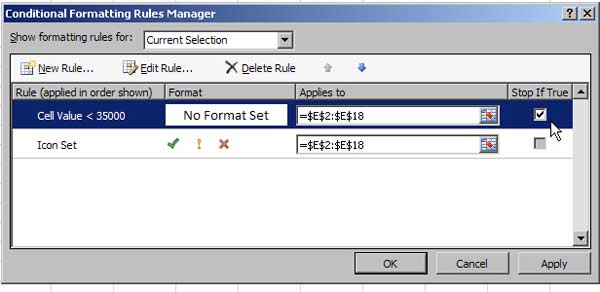
Go back to Home, Conditional Formatting, Manage Rules. The most recent rule (Cell Value < 35000) will be on top. Click the checkbox to Stop If True: