
Five Things to Know When Upgrading to Excel 2007
February 15, 2007
Here are five must-know techniques for Excel 2007
-
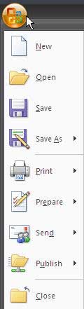
That round icon in the upper left corner is the File menu. Yes – Microsoft hid all of the most important menu commands behind a weird icon instead of behind the word “File”.
Click the icon to access trivial commands like Save, Print, and Close. After I installed Excel 2007 on my wife's machine without any training, she searched every ribbon tab looking for a way to print. I believe her exact quote was "who would hide something important like PRINT behind a button with no words!!!".
-
Excel offers 1.1 million rows, but if you open an old file, you only get 65 thousand rows. This is because you are in compatibility mode. Microsoft wants you to click the Office Icon and choose Convert. HOWEVER, I hate this method. When you use the convert command, Microsoft erases the old Excel 2003 file. If you would rather have both versions, then follow these steps:
- Click the Office Icon. Choose Save As - Excel Workbook.
- In the Save As dialog, give the workbook a name and click Save.
- Close the workbook.
- Re-open the workbook.
Yes - those last two steps are the ones that actually allow you to see 1.1 million rows.
-
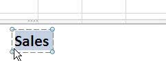
Many cool formatting tools are on an invisible toolbar called the Mini Toolbar. In order to make the Mini Toolbar visible, you have to move your mouse towards the invisible toolbar!
Maybe this is only my problem, but I select text from right to left. So, naturally, my mouse is moving from the top right to the bottom left of text when I select it. The MSFT intelligence says that to make the Mini Toolbar appear, you have to move the mouse up and to the right from your selection. When you move up and to the right, the mini toolbar solidifies. When you move down or to the left, the mini toolbar becomes completely invisible. In this image, I just selected text from the top right to the bottom left. Can YOU see the toolbar?
If you know to move up and to the right, the mini toolbar starts to materialize.
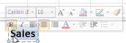
There are a lot of great icons there, floating right by your selection, you just have to know to move up and to the right to make it appear.
-
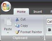
Customize the Quick Access Toolbar to have all of your favorite commands available all the time. One problem with the ribbon is that all of the important commands on the Home ribbon will not be visible if you select one of the other 7 ribbon tabs. If you have favorite commands that you use all the time, add them to the Quick Access Toolbar. The Quick Access Toolbar starts out above the ribbon:
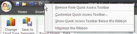
If you want the toolbar closer to your spreadsheet, right-click and choose Show Quick Access Toolbar below the Ribbon.
To add a favorite icon to the Quick Access Toolbar, right-click the Icon and choose Add to Quick Access Toolbar.
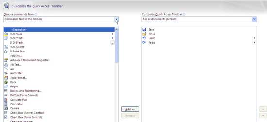
To have full control over the QAT, right-click the QAT and choose Customize Quick Access Toolbar. You can now move any commands to the QAT, re-order the icons on the QAT, and specify that certain icons should only appear when the current workbook is open.
Tip
In the Choose Commands From dropdown, select "Commands Not in the Ribbon". You will find a number of useful but obscure commands there that never found a home anywhere on the ribbon. For example, if you are looking for the Text to Speech commands to pull off my evil April Fool's joke in Excel, they have been banished to "Command Not in the Ribbon".
- The formula bar is now scrollable. If you select the formula bar and it doesn’t show your whole formula, you can scroll it into view. This prevents long formulas from covering up row 1 of the spreadsheet. Just realize that you may not be seeing the entire formula in the formula bar. Use the scroll buttons at the right edge of the formula bar.
- Live Preview will show you results before you actually click them. The gotcha, though, is that you then actually have to click them in order to see the results.