
Tables in Excel 2007
February 23, 2007
In Excel 2003, Microsoft introduced List functionality (Ctrl+L). They've improved and replaced this in Excel 2007 with table functionality. Most spreadsheets contain data in a tabular format - headings across the top and each row containing a new record. If you have data in a tabular format, select a cell and press Ctrl+T to convert the range to a table.
Once you have a table defined, you can use the tools in the Table Tools Design ribbon:
-
Add totals with a single click by choosing the Total Row checkbox in the Table Style Options group.
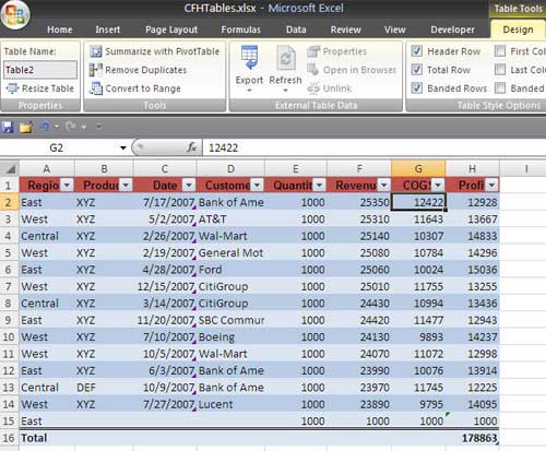
- Add a new record in the blank row under the table and the table will expand to include the new row.
-
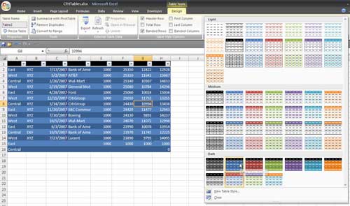
Format with one of 60 different color schemes in the Table Styles gallery. Note that the 6 checkboxes in the Table Style Options group will modify look of each style. (This gallery supports Live Preview - just hover over a style to preview it in the worksheet.
-
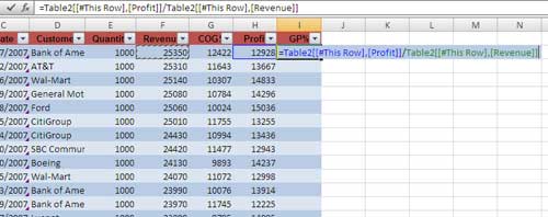
Enter a formula in the first row of a table and have the formula automatically copy to every row. Tip: format cell I2 as a percentage before you enter the formula in I2. Here is the spreadsheet just before I press Enter:
-
Here is the spreadsheet after I click Enter. Excel has filled in the formulas to the bottom of the table.
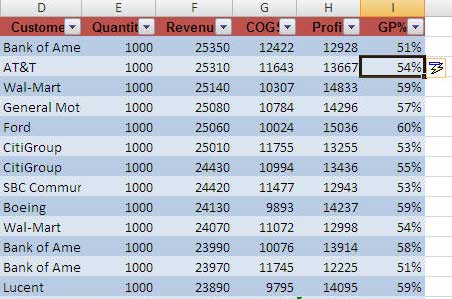
Notice in the last image that Excel uses a new table nomenclature for formulas that point to a table. This replaced the old Natural Language Formulas that have been in Excel for several versions.
One advantage of tables is that any charts or pivot tables that are built based on a table will automatically expand to include new data when the table expands.
The tip in this show is from Excel 2007 Miracles Made Easy E-Book