
Track Your Next Loan in Excel
October 22, 2007
While I have shown how to use the PMT function in past shows, today I want to show how to create an amortization table.
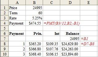
- Build the input section of the worksheet as shown in A1:B3. The formula for cell B4 is shown in red in C4.
- Enter the headings shown in Row 6.
- The initial balance in D7 is a formula that points to B1.
- In A8:A67, enter the numbers 1 through 60. (Tip: Enter 1 in A8. Select A8. Hold down the Ctrl key while you drag the Fill Handle downwards. The Fill Handle is the square dot in the lower right corner of the cell).
-
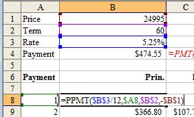
Use the PPMT function to calculate interest principal for any given payment in column B. Enter this formula in B8:
-
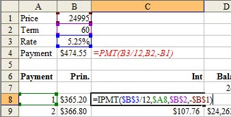
Use the IPMT function to calculate interest for any given payment in column C. Enter this formula in CB8:
- The formula in D8 is =D7-B8.
- Copy B8:D8 down to rows 9 through 67
One tip mentioned in the show is to replace column A with a reference to ROW(A1). You can change the formula in B8 to be =PPMT($B$3/12,ROW(A1),$B$2,-$B$1).