Excel Sort With a Formula Using SORT and SORTBY

September 25, 2018 - by Bill Jelen

This week at the Ignite Conference in Orlando Florida, Microsoft debuted a series of new, easier array formulas in Excel. I will be covering these new formulas every day this week, but if you would like to read ahead:

• Monday covered the new =A2:A20 formula, the SPILL error, and the new SINGLE function required in place of Implicit Intersection
• Today will cover SORT and SORTBY
• Wednesday will cover FILTER
• Thursday will cover UNIQUE
• Friday will cover SEQUENCE and RANDARRAY functions

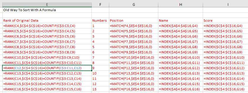
Sorting with a Formula in Excel used to require an insane combination of formulas. Take a look at this data which will be used throughout this article.

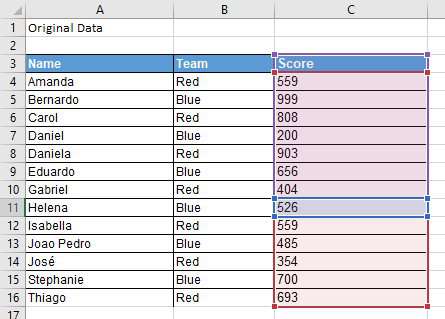
In order to sort this with a formula before this week, you would just have to knock out RANK, COUNTIF, MATCH, INDEX and INDEX. Once you finished this set of formulas, you would be ready for a nap.

Joe McDaid and his team have brought us SORT and SORTBY.

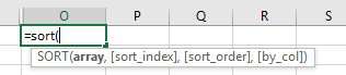
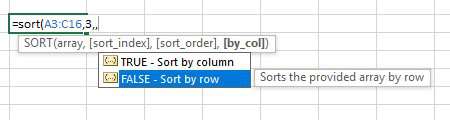
Let's start with SORT. Here is the syntax =SORT(Array, [Sort Index], [Sort Order], [By Column])

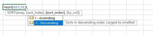
Let's say you want to sort A3:C16 by the Score field. Score is the third column in the array, so your Sort Index will be 3.

The choices for the Sort Order are 1 for ascending or -1 for descending. I am not complaining, but there will never be support for Sort by Color, Sort by Formula, or Sort by Custom List using this function.

The forth argument is going to be rarely used. It is possible in the Sort dialog to sort by column instead of rows. 99.9% of people sort by rows. If you need to sort by column, specify True in the final argument. This argument is optional and defaults to False.

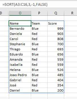
Here are the results of the formula. Thanks to the new calc engine, the formula spills into adjacent cells. One formula in O2 produces this solution.

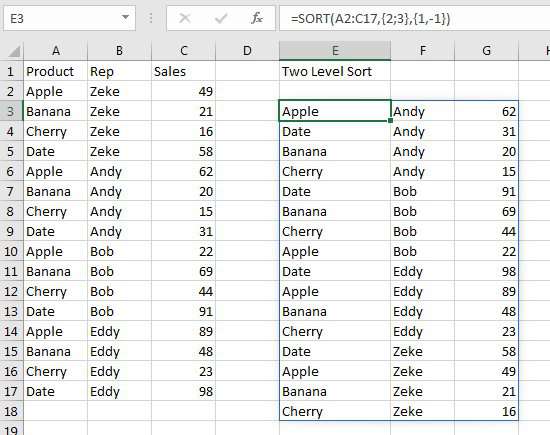
What if you need a two-level sort? Sort by column 2 ascending and column 3 descending? Supply an array constant for the 2nd and 3rd arguments: =SORT(A2:C17,{2;3},{1;-1})

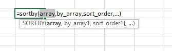
The SORTBY function lets you sort by something not in the results

The SORTBY function syntax is =SORTBY(array, by_array1, sort_order1,)

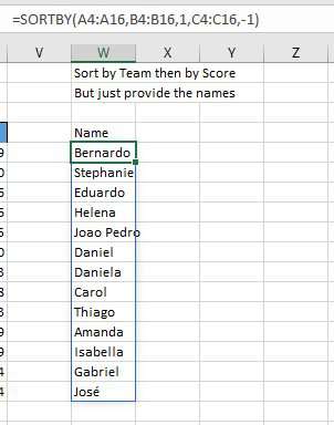
Going back to the original data. Say you want to sort by Team then Score, but only show the names. You could use SORTBY as shown here.

Random Drug Testing and Random With No Repeats

Difficult scenarios like Random Drug Testing and Random with No Repeats become mind-numbingly simple when you combine SORT with RANDARRAY.

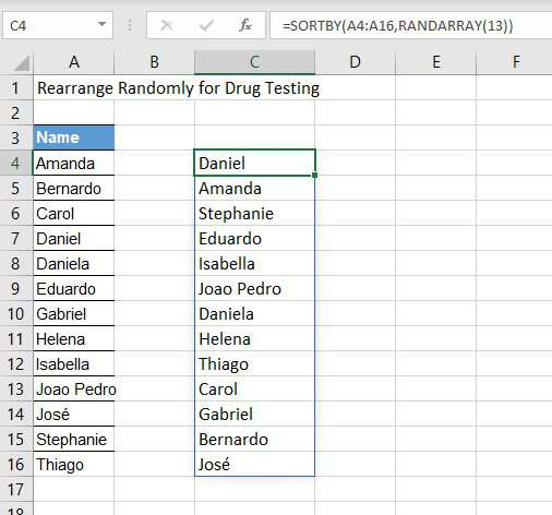
In the figure below, you want to sort the 13 names randomly without repeats. Use =SORTBY(A4:A16,RANDARRAY(13)). Read more about RANDARRAY on Friday.

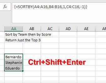
Is Ctrl + Shift + Enter completely dead? No. There is still a use for it. Let's say you wanted only the top 3 results from the SORT function. You could select three cells, type the SORT function and follow it with Ctrl + Shift + Enter. This will prevent the results from spilling beyond the bounds of the original formula.

Watch Video

Title Photo: Farsai C. on Unsplash