Excel Vlookup Index Match
April 02, 2002 - by Bill Jelen
If you've been reading Excel tips for a while, you have invariably found someone who talks about using Excel INDEX() & MATCH() functions instead of Excel VLOOKUP. Speaking for myself, it was always too hard to try and master TWO new functions simultaneously. But, it IS a cool trick. Give me five minutes and I will try to explain it in simple English.
The 30 second review of VLOOKUP
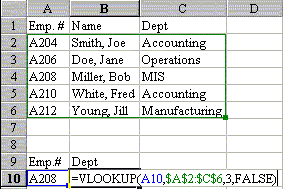
Say you have a table of employee records. The first column is an employee number, and the remaining columns are various data about the employee. Any time you have an employee number in the worksheet, you can use VLOOKUP to return a specific datum about the employee. The syntax is VLOOKUP(value,data range,col no.,FALSE). It says to Excel, "Go to the data range. Find a row that has (value) in the first column of the data range. Return the (col no.)th value from that row. Once you get the hang of it, it is very simple and powerful.
The Problem
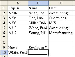
One day, you have a situation where you have the employee name, but need the employee number. In the following image, you have a name in A10 and need to find the employee number in B10.
When the key field is to the right of the data you want to retrieve, VLOOKUP will not work. If only the VLOOKUP would accept -1 as the column number, there would be no problem. But, it doesn't. One common solution is to temporarily insert a new column A, copy the column of names to the new column A, populate with VLOOKUP, Paste Special Values, then delete the temporary column A. Excel pros can probably do this move in their sleep.
I am going to suggest you take the challenge and try to use this single step method. Yes, you will have to tack the formula up on your wall for a few weeks, but you did that with VLOOKUP a long time ago, too, didn't you?
I think the reason this is so difficult is that you are using two functions which you probably never used before. So, let me break it down into two pieces.
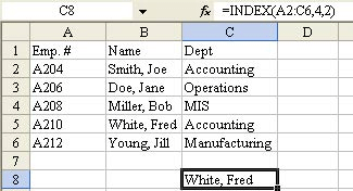
First, there is the INDEX() function. This is a horribly named function. When someone says "index", it does not conjure up anything in my mind that is similar to what this function does. Index requires three arguments.
=INDEX(data range, row number, column number)
In English, Excel goes to the data range and returns you the value in the intersection of the (row number)th row and the (column number)th column. Hey, think about it - this is pretty simple, right? =INDEX($A$2:$C$6,4,2) will give you the value in B5.
Applying INDEX() to our problem, you can figure that to return the employee number from the range, you would use this: =INDEX($A$2:$A$6,?,1). Actually, this piece of it seems so trivial that it seems useless. But, when you replace the question mark with a MATCH() function, you have the solution.
Here is the syntax:
=MATCH(Value, Single-column data range, FALSE)
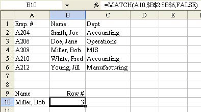
It tells Excel, "Search the data range and tell me the relative row number where you find a match for (data). So, to find which row has the employee in A10, you would use =MATCH(A10,$B$2:$B$6,FALSE). Yes, this is more complex than Index, but it should be right up the alley of VLOOKUP pros. If A10 contains "Miller, Bob" then this MATCH will return that he is in the 3rd row of the range B2:B6.
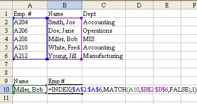
There it is - the MATCH() function tells the Index function which row to look in - you are done. Take the Index function, replace our question mark with the MATCH function, and you can now do the equivalent of VLOOKUPs when the key field is not in the left column. Here is the function to use:
=INDEX($A$2:$A$6,MATCH(A10,$B$2:$B$6,FALSE),1)
The sticky note on my wall actually shows it as two lines. First I wrote out the explanation for MATCH(). Below that I wrote the explanation for INDEX(). I then drew a funnel shape between the two to indicate that the MATCH() function drops in to the 2nd argument of the INDEX() function.
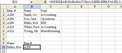
The first few times I had to do one of these, I was tempted just to slam a new temporary column A in there, but went through the pain of doing it this way instead. It is faster, and requires less manipulation. So, the next time you are wishing you could put a negative number in the VLOOKUP function, try this strange combination of INDEX and MATCH to solve your problems.

