
Pivot Table Tricks
August 06, 2005
To try this tip on your own computer, download and unzip CFH231.zip.
Pivot Tables are Excel's most powerful feature. Other tips at this site discuss pivot tables, but today's show talks about two interesting uses for Pivot Tables. First, you can use a pivot table to come up with a unique list of values from a field. Second, you can use a pivot table to show the percentage of items in a row.
The dataset has 10,000+ rows of sales data. There are columns for customer, product, month, and quantity sold.

Finding Unique Values
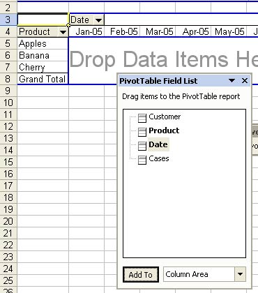
The traditional way to find unique values from a list is to use the Data - Filter - Advanced Filter command. However, you can also create a unique list of values with a pivot table. Select a single cell in the dataset. From the menu, choose Data - PivotTable and PivotChart Report. Click Finish. You will be presented with a blank pivot table as shown below.

To get a unique list of customers, select the Customer field and press the Add To Row Area button.

If you count, that was a total of four clicks. You can now copy cells A5:A28 to another worksheet and you have a unique list of customers.

Calculating Percentage of Total
Return to your original dataset and select a single cell. From the menu, select Data - PivotTable & Pivot Chart Report. Click Finish to create a blank pivot table.
In the PivotTable Field List, choose Product and click Add To Row Area.
Next, choose the Date field. Change the dropdown at the bottom of the field list to be column area and click the Add to button.
Choose the Cases field. Change the dropdown to Data area. Click the Add to button. The resulting pivot table will show sales by product and month.
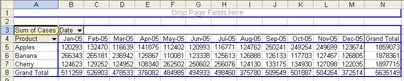
Although this report is a summary of 10,000 rows of data, it is still a confusing jumble of numbers. It is really hard to spot trends in the data. When do Bananas sell best? It is hard to tell.
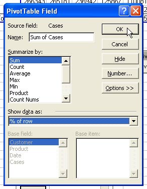
Double-click the Sum of Cases button in cell A3 to display the PivotTable Field dialog. The dialog gives you a few settings that you rarely need to change. However, choose the Options button to see more options.

The expanded dialog indicates that you are displaying the data as Normal.

Select the Show Data As dropdown. There are options for:
- Normal
- Difference From
- % of
- % Difference Of
- Running Total In
- % of Row
- % of Column
- % of Total
- Index
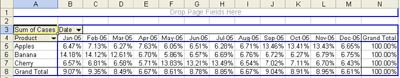
For today's analysis, choose % of Row. The Base Field and Base Item are not relevant for the % of Row, so those options are greyed out. Choose OK to close the dialog box and return to the pivot table.
In the resulting pivot table, you can see that Banana sales are strongest in January through February. Apples do the best in September through November and Cherries do well in May through July.
Although Pivot Tables generally take four clicks to create, they have many additional features that allow for even more powerful analyses. People are often surprised that Michael Alexander and I could fill 250 pages about one feature of Excel, but when you consider all of the various options in a pivot table, it does merit a complete book.
Tips from this episode are from Pivot Table Data Crunching.