Column chart

[leebradley1977]

Hi All - I've been chasing this for days and I know I'm missing something simple. If any gurus could help I would be eternally grateful.

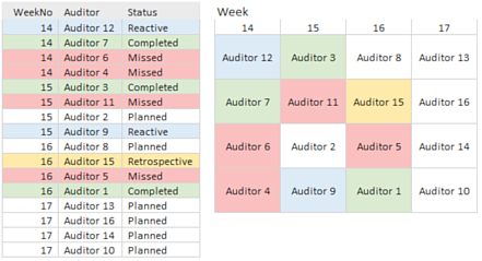
Basically - I have a list of auditors as per below:

As you can see in Column A I have a week number - in B its the Auditor, and C it the status.

Theres some basic conditional formatting on the sheet which highlights the row in the appropriate colour depending on the status of the audit. Columns B and C entries are selected from drop down lists.

There are a total of 25 auditors in the list and 5 status items which generate a colour

Planned = no fill / white
Completed= Green
Missed = Red
Retrospective = Orange
Reactive = Blue

The list grows each month as I plan in more audits for the team.

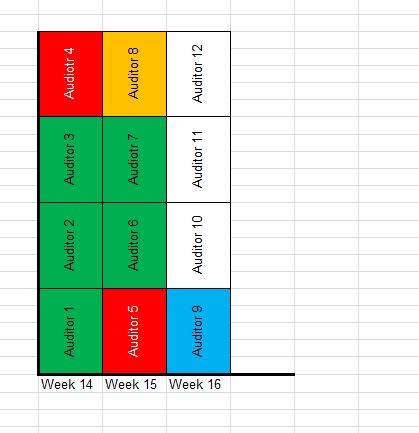
What I'm looking to create is a column chart which is split into 4 sections for each week (a bit like a stacked chart) - in each section I want to put the auditor name and I want the colour to match the status.


Is this doable?. I'm going around in circles and driving myself insane.

 

[leebradley1977]

Re: Help with a column chart

for clarity - a crude mockup of what I'm trying to get to:

 

[leebradley1977]

Re: Help with a column chart

Hi All. Can anyone help?

 

[thisoldman]

Re: Help with a column chart

Book1
	A	B	C	D	E	F	G	H
1	WeekNo	Auditor	Status		Week
2	14	Auditor 12	Reactive		14	15	16	17
3	14	Auditor 7	Completed		2	6	10	14
4	14	Auditor 6	Missed		Auditor 12	Auditor 3	Auditor 8	Auditor 13
5	14	Auditor 4	Missed		Reactive	Completed	Planned	Planned
6	15	Auditor 3	Completed		3	7	11	15
7	15	Auditor 11	Missed		Auditor 7	Auditor 11	Auditor 15	Auditor 16
8	15	Auditor 2	Planned		Completed	Missed	Retrospective	Planned
9	15	Auditor 9	Reactive		4	8	12	16
10	16	Auditor 8	Planned		Auditor 6	Auditor 2	Auditor 5	Auditor 14
11	16	Auditor 15	Retrospective		Missed	Planned	Missed	Planned
12	16	Auditor 5	Missed		5	9	13	17
13	16	Auditor 1	Completed		Auditor 4	Auditor 9	Auditor 1	Auditor 10
14	17	Auditor 13	Planned		Missed	Reactive	Completed	Planned
15	17	Auditor 16	Planned
16	17	Auditor 14	Planned
17	17	Auditor 10	Planned
Sheet1

Cell Formulas
Range	Formula
E3	=MATCH(E$2, $A:$A, 0) + (ROW() - ROW($I$3)) / 3
E4	=INDEX($B:$B, E3)
E5	=INDEX($C:$C, E3)

Each unit block has three formulas—it will be painful to copy and paste the block if your chart is large.

Two cells per block, the first row and the third row, have their results hidden using custom number formatting. Select the cells, Ctrl+1, then on the Number tab select Custom. In the text box labeled "Type:", enter three semicolons, ";;;", using no spaces or quotation marks.

Conditional formatting rules apply to all the blocks. In the example, each rule applies to E3:H14.
=ISNUMBER(MATCH("Completed", E3:E5, 0)) :: green
and similarly, for each word in your list.

The workbook can be downloaded from: https://www.dropbox.com/s/okkqw4nma107yxx/leebradley.xlsx?dl=0