I can't get the conditional formatting to work even though the index formula works in a cell.
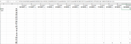
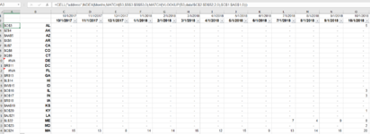
Here is my formula: =CELL("address",INDEX(Months,MATCH(B3,$B$3:$B$53,0),MATCH(VLOOKUP(B3,data!$C$2:$D$52,2,0),$C$1:$AS$1,0)))
I copied this formula into the CF from cell C3 and applied it to my range, months.


In one of my many attempts, I got several cells to turn green, however they were before the start date and not on every row. I deleted it, so I don't know how I got that even to work incorrectly.

I'd like each starting cell (O3 for row 1) to be highlighted, as well as the corresponding location of the index formula result for each row of my range. I didn't find an acceptable way to make the cell reference relative. Is this the problem?
I am hoping to do the entire calculation in the CF rather than use a step by step approach such as I have now in column A (illustration purposes).
Thank you for your time,
Tifne
Here is my formula: =CELL("address",INDEX(Months,MATCH(B3,$B$3:$B$53,0),MATCH(VLOOKUP(B3,data!$C$2:$D$52,2,0),$C$1:$AS$1,0)))
I copied this formula into the CF from cell C3 and applied it to my range, months.
In one of my many attempts, I got several cells to turn green, however they were before the start date and not on every row. I deleted it, so I don't know how I got that even to work incorrectly.
I'd like each starting cell (O3 for row 1) to be highlighted, as well as the corresponding location of the index formula result for each row of my range. I didn't find an acceptable way to make the cell reference relative. Is this the problem?
I am hoping to do the entire calculation in the CF rather than use a step by step approach such as I have now in column A (illustration purposes).
Thank you for your time,
Tifne