Hi All,
I've had a look around this forum and was unable to find an answer to my question. Essentially I have a table that depending on the value of a list item, shows 3 different sets of data in the same cells.
I want to apply conditional formatting to results on just one of the list item results cells. I have had success getting the red, amber and green styles applied for a single cell on the value, but I am having trouble scaling this to cover the entire table.
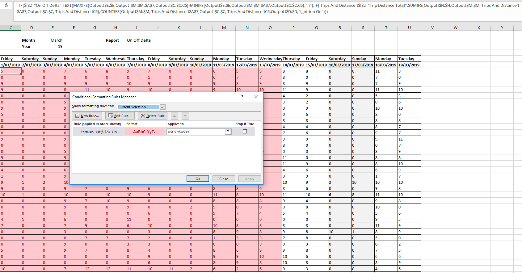
The formula in each cell is as per below, I know it isn't as optimised as it could be however it does get the job done.
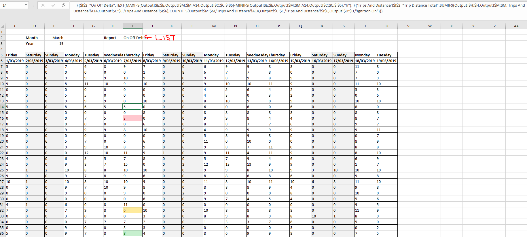
The list values are "Trip Distance Total, Ignition Started, On Off Delta". The results of On Off Delta are an shown as an hour count using =TEXT(cell,"h"), typically between 1 and 15.
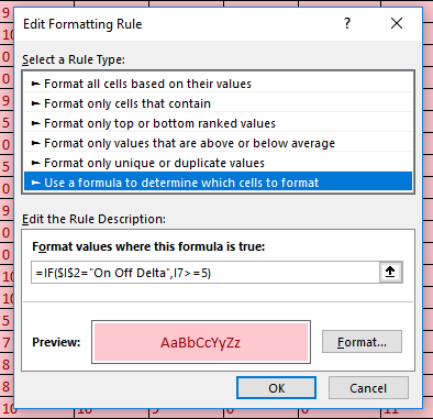
The conditional formatting style I have been using as per below (I2 is the list value cell)
Red -
- I16 is a random cell in the table that has a value lower than 5
Amber -
Green -
The condition formula above applies only to the cell that is referred to that the end of the code (the one it is checking the value against). I am struggling to think of a way to make this scale-able so that I do not need to go through and manually add 3 conditional formatting rules on each cell of the table.
Hopefully this explanation of this issue is thorough enough, please let me know if you need anything further! Here is a snap showing the formula and cell values to give an idea.
Cheers,
Mat
I've had a look around this forum and was unable to find an answer to my question. Essentially I have a table that depending on the value of a list item, shows 3 different sets of data in the same cells.
I want to apply conditional formatting to results on just one of the list item results cells. I have had success getting the red, amber and green styles applied for a single cell on the value, but I am having trouble scaling this to cover the entire table.
The formula in each cell is as per below, I know it isn't as optimised as it could be however it does get the job done.
Code:
=IF($I$2="On Off Delta",TEXT(MAXIFS(Output!$E:$E,Output!$M:$M,$A$7,Output!$C:$C,C6)-MINIFS(Output!$E:$E,Output!$M:$M,$A$7,Output!$C:$C,C6),"h"),IF('Trips And Distance'!$I$2="Trip Distance Total",SUMIFS(Output!$H:$H,Output!$M:$M,'Trips And Distance'!$A$7,Output!$C:$C,'Trips And Distance'!C6),COUNTIFS(Output!$M:$M,'Trips And Distance'!$A$7,Output!$C:$C,'Trips And Distance'!C6,Output!$D:$D,"Ignition On")))The list values are "Trip Distance Total, Ignition Started, On Off Delta". The results of On Off Delta are an shown as an hour count using =TEXT(cell,"h"), typically between 1 and 15.
The conditional formatting style I have been using as per below (I2 is the list value cell)
Red -
Code:
=IF($I$2="On Off Delta",$I$16>=5)Amber -
Code:
=IF($I$2="On Off Delta",$I$32>5,$I$32<7)Green -
Code:
=IF($I$2="On Off Delta",$I$36<=7)The condition formula above applies only to the cell that is referred to that the end of the code (the one it is checking the value against). I am struggling to think of a way to make this scale-able so that I do not need to go through and manually add 3 conditional formatting rules on each cell of the table.
Hopefully this explanation of this issue is thorough enough, please let me know if you need anything further! Here is a snap showing the formula and cell values to give an idea.
Cheers,
Mat
")