Employees performance chart

[Quintrala]

Good morning. It's my first time seeking help here. I have an Excel spreadsheet which has attendance reports for all employees working in the company. I want to create a pie chart which shows the percentage of good attendance, late arrivals, leaving early and absences per person each week and another for the same data per all employees each week. I have created totals for each value for each employee per each day (H2 to J7 in the image). As well as daily totals for all employee (B10 to G13 in image).

The spreadsheet looks as below.

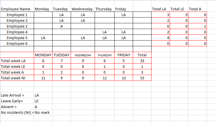
I want to know how to add the info into a pie chart since I have been following regular pie chart creation process and is not creating what I need but only adding one of the values instead of all.

Eventually I want to use the pie charts to create a per month and yearly report as well.

Can someone help me?

Thanks in advance for the help!

 

[oldbrewer]

why is total week LA for monday = 6

and is pie chart for each day? as you cant have mon to fri with 4 scores for each on a pie chart

 

[Quintrala]

why is total week LA for monday = 6

I did not add up real totals for the example in the picture. Just entered random numbers to create an image alike what I have since I need to protect employees names privacy.-

"and is pie chart for each day?"

First pie chart is mostly looking to compare employees on how they affect. An employee who is late every day will have a higher area of the pie while an employee with 0 lateness will not be even there. This one should use columns on far right area.

Second pie chart looks for how much each category affects the week. This would be seen trough the amount of late personnel per day. This one should use rows at the bottom of the sheet.

"as you cant have mon to fri with 4 scores for each on a pie chart."

Could not understand this part.

 

[oldbrewer]

last part - I thought you only wanted one pie chart ! but that is sorted now....

 

[oldbrewer]

	mon	tue	wed	thu	fri
emp1		LA	LA		LA		3	0.0000002	3
emp2		LA	LA				2	0.0000003	2
emp3		A					0	0.0000004	0		this last column is number of LA's
emp4				LA	LA		2	0.0000005	2		plus row number times .000001
emp5	LA		LA	LA	LA		4	0.0000006	4		(to sort out tie breaks)
emp6							0	0.0000007	0
		PUT THE LAST COLUMN IN DESCENDING ORDER
		1	4	emp5	4
		2	3	emp1	3	and use offset match to attach names
		3	2	emp4	2
		4	2	emp2	2	copy the numbers to right of name
		5	0	emp6	0
		6	0	emp3	0
		this makes a nice pie chart with emp5 and emp6 not actually showing
		but indicated as having zero value

<colgroup><col span="8"><col><col><col span="5"></colgroup><tbody>
</tbody>

 

[Quintrala]

I am so sorry. I'm a totally new user so I still don't get this since I don't even know what offset match is. Like I really need the step by step. I'm so sorry.

 

[oldbrewer]

No problem. Offset match is easy, start here, go down so many cells, go across so many cells. So offset(A1,7,5) returns the value in E8. Match just looks for a match in a row or column, So match(66,C1:H1,0) finds 66, say it is in E1 then the formula returns 2. So we can use match within offset.

offset(A3, match("red",A4:A10,0),match(66,C1:H1,0)) finds red then tracks across from C1 to H1 until it finds red. If 66 is in G1 and red is in A7 it goes to A7 and then across to column 7 ie G7.

I will post the formula I used later today.