Formula Questions, not sure how I should format the formula.

[Ancientfall]

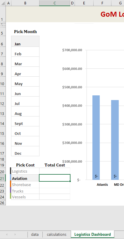
I have designed a dashboard for work, one of the sheets (called calculations) contains all of the raw figures and the other sheet I use displays the dashboard. I have the dashboard automatically change the chart depending on the month / specific figure selected (see below).

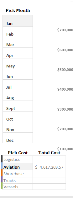
In the above picture, when someone clicks on the appropriate month/cost type (which is Cells B6-B17, Jan-Dec).

I would like excel to go to my calculations page and sum up the specific cost and put it into the total cost cell (which is cell C21). I'm not completely sure what formula I would need to use for this particular situation.

For example: If someone clicks the month of Feb. and they want to see Shorebase cost, I would like C22 to bring up the total cost for Feb. in that particular cell.

If you need more specific cells, I can provide them for you to make it easier to understand what I'm trying to convey.

 

[Oaktree]

Sounds like a textbook situation to have your table at the bottom be a pivot table and your Jan - Dec selections be a slicer linked to that pivot table.

If you're not familiar with them, there are tons of examples if you search Google for "add a slicer to a pivot table" or similar.

 

[Ancientfall]

Sounds like a textbook situation to have your table at the bottom be a pivot table and your Jan - Dec selections be a slicer linked to that pivot table.

If you're not familiar with them, there are tons of examples if you search Google for "add a slicer to a pivot table" or similar.

Is their a way to do it without converting all of my data to a pivot table? I've got quite a few formulas in my dashboard.

 

[Ancientfall]

Can anyone help with a formula instead of using the above-mentioned pivot/slicer example?

 

[Oaktree]

OK. If you don't like the pivot table idea, here are three other other strategies you could consider:

1) Apply a slicer (without the pivot table) to the data table. That will filter your data, and you can then use the =SUBTOTAL(9,range) formula which only sums cells not hidden by the filter.

2) Use option buttons for Jan - Dec and link them all to the same cell (e.g. E1). Then, set

F1 =INDEX({"Jan","Feb","Mar","Apr","May","Jun","Jul","Aug","Sep","Oct","Nov","Dec"},E1)

and finally use F1 within a formula like =SUMIF(month_range,F1,data_range)

3) Use a selection change event macro. If you don't want to add a slicer or an option button, you could right click on your sheet tab, select "view code", and paste the code below, and use the SUMIF as in #2 above:

Private Sub Worksheet_SelectionChange(ByVal Target As Range)
If Intersect(Target, Range("A1:A12")) Is Nothing Then End
[F1] = Target.Value
End Sub

 

[Ancientfall]

OK. If you don't like the pivot table idea, here are three other other strategies you could consider:

1) Apply a slicer (without the pivot table) to the data table. That will filter your data, and you can then use the =SUBTOTAL(9,range) formula which only sums cells not hidden by the filter.

2) Use option buttons for Jan - Dec and link them all to the same cell (e.g. E1). Then, set

F1 =INDEX({"Jan","Feb","Mar","Apr","May","Jun","Jul","Aug","Sep","Oct","Nov","Dec"},E1)

and finally use F1 within a formula like =SUMIF(month_range,F1,data_range)

3) Use a selection change event macro. If you don't want to add a slicer or an option button, you could right click on your sheet tab, select "view code", and paste the code below, and use the SUMIF as in #2 above:

Private Sub Worksheet_SelectionChange(ByVal Target As Range)
If Intersect(Target, Range("A1:A12")) Is Nothing Then End
[F1] = Target.Value
End Sub

Oak, thanks for the input, I apologize for making this more complicated than it should be. After looking at all three of the options I would like to perform the third option. So I went an inputted the macro information into the Worksheet SelectionChange.

This is what I currently have in my code for my worksheet:

Private Sub Worksheet_SelectionChange(ByVal Target As Range)
    If Not Application.Intersect(ActiveCell, [plstMonth]) Is Nothing Then
        [valMonthPicked] = ActiveCell.Value
    ElseIf Not Application.Intersect(ActiveCell, [plstCostElement]) Is Nothing Then
        [valCostPicked] = ActiveCell.Value
    ElseIf Not Application.Intersect(ActiveCell, [plstRigName]) Is Nothing Then
        [valRigPicked] = ActiveCell.Value
    End If
        If Intersect(Target, Range("C6:C17")) Is Nothing Then End
[C20] = Target.Value
End Sub

So, my months are cells C6:C17 and I'm not 100% sure what [F1] should be? Is that supposed to be whatever the cell # is for Logistics? I've attached my current cell structure for reference.

So should [F1] be where I input the =SUMIF(month_range,F1,data_range).

Let me know if you need more information. I really appreciate your help Oak!

 

[Oaktree]

Sounds like we're getting closer.

[F1] in my example was under the assumption that the only selection change you wanted to capture was the month. In that case, I was setting an unused F1 cell = to the selected month. That way, we could then use F1's value in a standard =SUMIF(month_range,F1,data_range) formula, noting that F1's value would change via macro whenever the selection changed.

... but, it sounds like your desire is a little more complicated than that.

From

Private Sub Worksheet_SelectionChange(ByVal Target As Range)
    If Not Application.Intersect(ActiveCell, [plstMonth]) Is Nothing Then
        [valMonthPicked] = ActiveCell.Value
    ElseIf Not Application.Intersect(ActiveCell, [plstCostElement]) Is Nothing Then
        [valCostPicked] = ActiveCell.Value
    ElseIf Not Application.Intersect(ActiveCell, [plstRigName]) Is Nothing Then
        [valRigPicked] = ActiveCell.Value
    End If
        If Intersect(Target, Range("C6:C17")) Is Nothing Then End
[C20] = Target.Value
End Sub

One small thing: you might change ActiveCell to instead be Target. Since you have the target variable available to you through the SelectionChange event, it's a little cleaner to use that instead of activecell.

It looks like you want to assign the selected value to one of three cells: valMonthPicked, valCostPicked, or valRigPicked. Those essentially replace what I was using F1 for in my example.

I think the same principle holds though. You could use =SUMIF or =SUMPRODUCT... or whatever conditional aggregation formula you wanted, referencing those val...Picked cell references as inputs to the formulas. The macro would change those input values accordingly, and your formulas would recalculate accordingly.