Match 2 Criteria on multiple sheet and return a value

[Yvonne Ng]

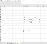
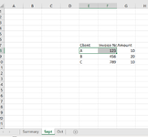
I have data sheet namely Sept, Oct.
I want to create a summary page to see how much I've been bill on that particular invoice.
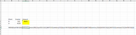
I try used index and match function for multiple sheet, but not successful.

Please illustrate and advise.
Attached file for reference.

 

[Yvonne Ng]

I have 3 data base here, showing Sept, oct, Nov, and I have 3 seperate summary page for 3 different client. I want retreve the amount on different month sheet and input into client's summary.
this is exactly what i need

I need a formular that can lookup all the month sheet and into the amount into individual client summary sheet

 

[BigBeachBananas]

I have 3 data base here, showing Sept, oct, Nov, and I have 3 seperate summary page for 3 different client. I want retreve the amount on different month sheet and input into client's summary.
this is exactly what i need

It's not different than what I showed already. You would have 12 help columns for each month for each Client sheet.

EDIT: The numbers came out wrong because I didn't input values in Oct sheet.

Book2
	A	B	C	D	E	F	G
1	Client	Invoice	Sept	Oct	Dec	Amount	Comment
2	A	A123	10	0	0	10	Found In Sept Sheet
3	A	424	0	10	0	10	Found In Oct sheet
4	A	532	0	0	0	0
ClientA

Cell Formulas
Range	Formula
C2:E4	C2	=IFERROR(INDEX(INDIRECT("'" &C$1& "'!$C2:C5"),MATCH($A2&$B2,INDIRECT("'" & C$1 & "'!$A$2:$A$5") &INDIRECT("'" & C$1 & "'!$B$2:$B$5"),0)),0)
F2:F4	F2	=SUM(C2:E2)

Book2
	A	B	C	D	E	F	G
1	Client	Invoice	Sept	Oct	Dec	Amount	Comment
2	C	567	0	30	0	30	Found in Oct Sheet
3	C	A567	30	0	0	30	Found in Sept Sheet
ClientC

Cell Formulas
Range	Formula
C2:D3	C2	=IFERROR(INDEX(INDIRECT("'" &C$1& "'!$C2:C5"),MATCH($A2&$B2,INDIRECT("'" & C$1 & "'!$A$2:$A$5") &INDIRECT("'" & C$1 & "'!$B$2:$B$5"),0)),0)
F2:F3	F2	=SUM(C2:E2)

 

[Yvonne Ng]

It's not different than what I showed already. You would have 12 help columns for each month for each Client sheet.

Book2
	A	B	C	D	E	F	G
1	Client	Invoice	Sept	Oct	Dec	Amount	Comment
2	A	A123	10	0	0	10	Found In Sept Sheet
3	A	424	0	0	0	0
4	A	532	0	0	0	0
ClientA

Cell Formulas
Range	Formula
C2:E4	C2	=IFERROR(INDEX(INDIRECT("'" &C$1& "'!$C2:C5"),MATCH($A2&$B2,INDIRECT("'" & C$1 & "'!$A$2:$A$5") &INDIRECT("'" & C$1 & "'!$B$2:$B$5"),0)),0)
F2:F4	F2	=SUM(C2:E2)

Book2
	A	B	C	D	E	F	G
1	Client	Invoice	Sept	Oct	Dec	Amount	Comment
2	C	567	0	0	0	0
3	C	A567	30	0	0	30	Found in Sept Sheet
ClientC

Cell Formulas
Range	Formula
C2:D3	C2	=IFERROR(INDEX(INDIRECT("'" &C$1& "'!$C2:C5"),MATCH($A2&$B2,INDIRECT("'" & C$1 & "'!$A$2:$A$5") &INDIRECT("'" & C$1 & "'!$B$2:$B$5"),0)),0)
F2:F3	F2	=SUM(C2:E2)

But i only want to have the amount showing in one column only regardless of month.

 

[BigBeachBananas]

But i only want to have the amount showing in one column only regardless of month.

Then just hide the month and only show the Amount column? Or if you just want 1 formula you're welcome to combine each of those individual monthly formulas into 1, it would be very massive.

 

[Yvonne Ng]

Then just hide the month and only show the Amount column? Or if you just want 1 formula you're welcome to combine each of those individual monthly formulas into 1, it would be very massive.

yes, one formula to conbined all. this is exact what i need.

 

[BigBeachBananas]

yes, one formula to conbined all. this is exact what i need.

Here's the formula for 1 month. Replace "Sept" with other months and sum them all in 1 formula.

=IFERROR(INDEX(INDIRECT("'Sept" & "'!$C2:C5"),MATCH($A2&$B2,INDIRECT("Sept"  & "'!$A$2:$A$5") &INDIRECT("Sept" & "'!$B$2:$B$5"),0)),0)

 

[Yvonne Ng]

Here's the formula for 1 month. Replace "Sept" with other months and sum them all in 1 formula.

=IFERROR(INDEX(INDIRECT("'Sept" & "'!$C2:C5"),MATCH($A2&$B2,INDIRECT("Sept"  & "'!$A$2:$A$5") &INDIRECT("Sept" & "'!$B$2:$B$5"),0)),0)

I got a 0 instead of 10.
did i miss out anything?

Client	Invoice	Amount
A	A123	0​
A	424
A	532

 

[Yvonne Ng]

I got a 0 instead of 10.
did i miss out anything?

Client	Invoice	Amount
A	A123	0​
A	424
A	532

=IFERROR(INDEX(INDIRECT("'Sept" & "'!$C2:C5"),MATCH($A2&$B2,INDIRECT("Sept" & "'!$A$2:$A$5") &INDIRECT("Sept" & "'!$B$2:$B$5"),0)),0)
the formula i key in.

 

[BigBeachBananas]

=IFERROR(INDEX(INDIRECT("'Sept" & "'!$C2:C5"),MATCH($A2&$B2,INDIRECT("Sept" & "'!$A$2:$A$5") &INDIRECT("Sept" & "'!$B$2:$B$5"),0)),0)
the formula i key in.

We actually don't need the INDIRECT anymore. Try this:

=IFNA(INDEX(Sept!$C$2:$C$4,MATCH(ClientC!$A2&ClientC!$B2,Sept!$A$2:$A$4&Sept!$B$2:$B$4,0)),0)

Make sure the reference matches.

 

[Yvonne Ng]

We actually don't need the INDIRECT anymore. Try this:

=IFNA(INDEX(Sept!$C$2:$C$4,MATCH(ClientC!$A2&ClientC!$B2,Sept!$A$2:$A$4&Sept!$B$2:$B$4,0)),0)

Make sure the reference matches.

=IFNA(INDEX(Sept!$C$2:$C$4,MATCH(A2&B2,Sept!$A$2:$A$4&Sept!$B$2:$B$4,0)),0)
Its work for the data search for sept, but i try add for oct , the formular :
=IFNA(INDEX(Sept!$C$2:$C$4,MATCH(A3&B3,Sept!$A$2:$A$4&Sept!$B$2:$B$4,0))+INDEX(Oct!$C$2:$C$4,MATCH(A3&B3,Oct!$A$2:$A$4&Oct!$B$2:$B$4,0)),0)
Giving me A '0'. how should i corrrect the formula for the other months?