Public Sub UpdateTargetSheet()
Dim targetWS As Worksheet
Dim sourceWS As Worksheet
Dim targetLRow As Long
Dim sourceLRow As Long
Dim routeNum As Integer
Dim formulaStr As String
Set targetWS = Application.ThisWorkbook.Worksheets("Target")
Set sourceWS = Application.ThisWorkbook.Worksheets("Source")
targetLRow = targetWS.Cells(Rows.Count, 3).End(xlUp).Row
sourceLRow = sourceWS.Cells(Rows.Count, 3).End(xlUp).Row
If targetLRow > 1 Then targetWS.Range("A2:H" & targetLRow).Clear
If targetLRow > 1 Then targetWS.Range("L2:M" & targetLRow).Value = ""
targetLRow = 2 'reset target row to first row after clearing range
For i = 2 To sourceLRow
routeNum = sourceWS.Cells(i, 1) 'Grab current route
If IsEmpty(routeNum) = False Then
If sourceWS.Cells(i - 1, 1) <> routeNum Then
'If previous row has diff route num, add the dividing header
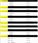
targetWS.Cells(targetLRow, 1) = sourceWS.Cells(i, 1)
targetWS.Range("A" & targetLRow & ":B" & targetLRow).Interior.ColorIndex = 6 ' Yellow
targetWS.Cells(targetLRow, 2) = "WarehouseDelays"
targetWS.Range("C" & targetLRow & ":H" & targetLRow).Interior.ColorIndex = 1 'Black
targetWS.Cells(targetLRow + 1, 3) = sourceWS.Cells(i, 2)
targetWS.Cells(targetLRow + 1, 4) = sourceWS.Cells(i, 3)
targetWS.Cells(targetLRow + 1, 6) = CStr(VBA.Left(sourceWS.Cells(i, 4).Text, 5)) & _
" - " & VBA.Left(sourceWS.Cells(i, 5).Text, 5)
formulaStr = "=IFERROR(Source!D" & i & " + 2/24, " & Chr(34) & " " & Chr(34) & ")"
targetWS.Cells(targetLRow + 1, 12) = formulaStr
formulaStr = "=IFERROR(Source!E" & i & " + 2/24, " & Chr(34) & " " & Chr(34) & ")"
targetWS.Cells(targetLRow + 1, 13) = formulaStr
targetWS.Cells(targetLRow + 1, 7) = VBA.Left(targetWS.Cells(targetLRow + 1, 12).Text, 5) & _
" - " & VBA.Left(targetWS.Cells(targetLRow + 1, 13).Text, 5)
targetLRow = targetLRow + 2
Else 'If previos is the same, enter in the data
targetWS.Cells(targetLRow, 3) = sourceWS.Cells(i, 2)
targetWS.Cells(targetLRow, 4) = sourceWS.Cells(i, 3)
targetWS.Cells(targetLRow, 6) = VBA.Left(sourceWS.Cells(i, 4).Text, 5) & _
" - " & VBA.Left(sourceWS.Cells(i, 5).Text, 5)
formulaStr = "=IFERROR(Source!D" & i & " + 2/24, " & Chr(34) & " " & Chr(34) & ")"
targetWS.Cells(targetLRow, 12) = formulaStr
formulaStr = "=IFERROR(Source!E" & i & " + 2/24, " & Chr(34) & " " & Chr(34) & ")"
targetWS.Cells(targetLRow, 13) = formulaStr
targetWS.Cells(targetLRow, 7) = VBA.Left(targetWS.Cells(targetLRow, 12).Text, 5) & _
" - " & VBA.Left(targetWS.Cells(targetLRow, 13).Text, 5)
targetLRow = targetLRow + 1
End If
Else
' Since the code above inserts separating rows
' based upon route num, no need to insert blanks on original sheet
End If
Next i
End Sub