VLOOKUP Duplicates First Item

[ScyberMhaster]

Good day!

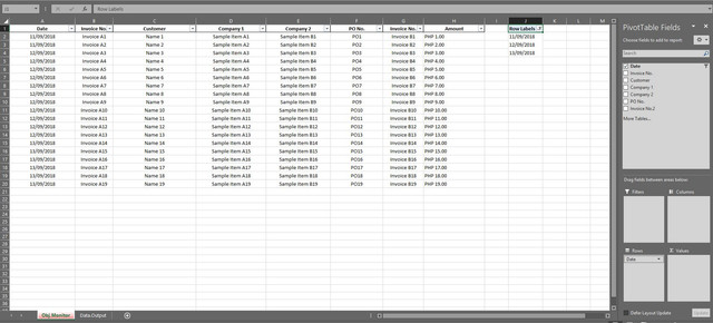
I badly need help with my workbook. I put sample values on my first sheet (Obj.Data), and I want to show it on my transmittal sheet (Data.Output). I used these functions:

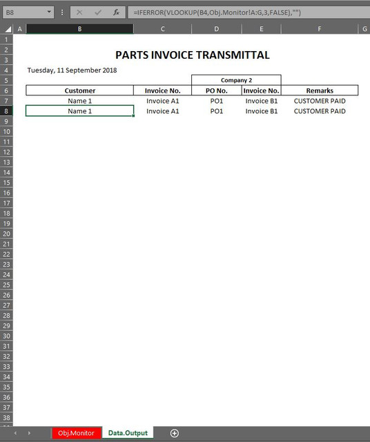
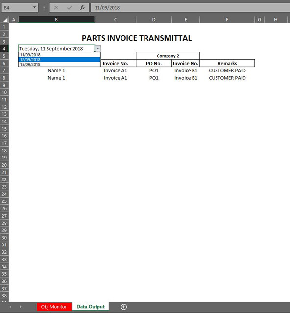
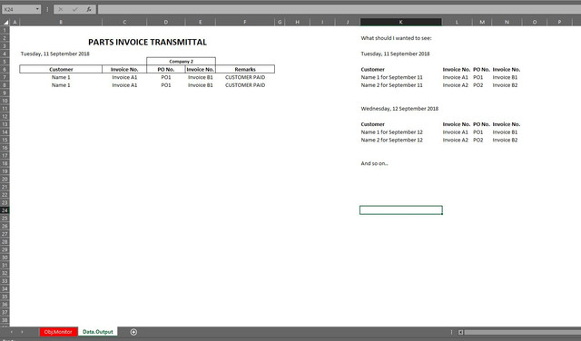
Pivot Table the Date, so I can remove duplicates or same dates. Then, I used Data Validation, and make the Pivot Table as source (date), to make drop-down list on my Data.Output. So I can choose the date which I wanted to display for my transmittal sheet. Then, I used VLOOKUP and IFERROR, to extract data from Obj.Data sheet. However, I have found error. The first row, is correct, but the second row only duplicates the first row.

B4 = Data Validation (Source = Pivot Table, Date)

ROW 1
=IFERROR(VLOOKUP(B4,Obj.Monitor!A:G,3,FALSE),"")
OUTPUT: Sample Name 1

ROW2
=IFERROR(VLOOKUP(B4,Obj.Monitor!A:G,3,FALSE),"")
OUTPUT: Sample Name 1
(Which should be Sample Name 2)

Please download the Excel File here.
https://ufile.io/e63fu

 

[Joe4]

Welcome to the Board!

In both cases you are looking up "B4", so they SHOULD return the same value.
If you want it to return a different value, you need to look up a different value (maybe "B5"?).

 

[ScyberMhaster]

Thank you sir for your reply!

The cell B4 is my Data Validation cell, which has a drop down list of my dates available via Pivot Table. Thus, should be the reference, I think.

 

[Joe4]

But it is only going to look up the value in the list that is currently selected.
The first argument of VLOOKUP is the value that you are looking up.

So if you have formulas in multiple cells looking up the same value within the same range and returning the same column, they should return the same value (how could they return anything different?).

If the change the value that you have in B4, all the formulas that are looking up B4 should change at the same time.

Here is an explanation of how VLOOKUP works: https://www.deskbright.com/excel/how-to-do-a-vlookup/

Maybe it would be better if you could actually post simple example and walk us through what you want to happen. You cannot upload files to this site. But there are tools you can use to post screen images. They are listed in Section B of this link here: http://www.mrexcel.com/forum/board-a...forum-use.html. Also, there is a Test Here forum on this board that you can use to test out these tools to make sure they are working correctly before using them in your question.

 

[ScyberMhaster]

Yes sir. That's right. Here, I wanted to illustrate how I wanted it to work:


Screenshot of my Data.Output Sheet

Cell B4 as Data Validation from my Pivot Table (Filtered = Date)

Screenshot of my Pivot Table

On the right side what I wanted to see sir for my Parts Invoice Transmittal. That whenever I choose specific date from my Data Validation Cell, it will extract data based on that date.

 

[Joe4]

Can you see any images in your post? I cannot.
Sometimes my workplace security blocks them, so I cannot tell if I cannot see them because they are being blocked, or if there are no images posted.

Note: One other thing about VLOOKUP - it can only return a single record. So if there are multiple records meeting the criteria, it will only ever return the first match (perhaps that is what you were asking?). So, you cannot use VLOOKUP to return multiple records.

 

[ScyberMhaster]

Yes, I see images on my post sir.

 

[Joe4]

OK. I cannot. I may be able to see them on my home computer, though I will not be on that for at least 8 hours.
Maybe someone else will see this reply in the meantime.

Also, note the last comment I made about VLOOKUP in my previous reply.

 

[Marcelo Branco]

You need an array formula in B7 copied down
=IFERROR(INDEX(Obj.Monitor!C$2:C$100,SMALL(IF(Obj.Monitor!$A$2:$A$100=$B$4,ROW(Obj.Monitor!C$2:C$100)-ROW(Obj.Monitor!C$2)+1),ROWS(B$7:B7))),"")
confirmed with Ctrl+Shift+Enter, not just Enter

Regular formula in C7 copied down
=IF(B7<>"",INDEX(Obj.Monitor!B:B,MATCH(B7,Obj.Monitor!C:C,0)),"")

Same idea for columns D to F

Hope this helps

M.

 

[ScyberMhaster]

You need an array formula in B7 copied down
=IFERROR(INDEX(Obj.Monitor!C$2:C$100,SMALL(IF(Obj.Monitor!$A$2:$A$100=$B$4,ROW(Obj.Monitor!C$2:C$100)-ROW(Obj.Monitor!C$2)+1),ROWS(B$7:B7))),"")
confirmed with Ctrl+Shift+Enter, not just Enter

Regular formula in C7 copied down
=IF(B7<>"",INDEX(Obj.Monitor!B:B,MATCH(B7,Obj.Monitor!C:C,0)),"")

Same idea for columns D to F

Hope this helps

M.

Thank you sir! It worked!!!