Weighted Average in Pivot Table

[Robert305]

Hi everyone,

I have a question which I just can't figure out. I have a pivot table and want to create a weighted average from that data. I have researched and people suggest to do this by using a calculated field. However, my data is structured differently, I have one measure per column. This is what my data looks like:

City	Product	Measure	Amount
Miami	Apple	Price	$4.0
Miami	Apple	Rating	50.0%
Miami	Pear	Price	$3.00
Miami	Pear	Rating	15.0%
Miami	Banana	Price	$13.00
Miami	Banana	Rating	85.0%
New York	Apple	Price	$2.00
New York	Apple	Rating	75.0%
New York	Pear	Price	$11.00
New York	Pear	Rating	15.0%
New York	Banana	Price	$9.00
New York	Banana	Rating	10.0%

This is what my pivot table looks like right now (I added the manually calculated weighted averages on the right):

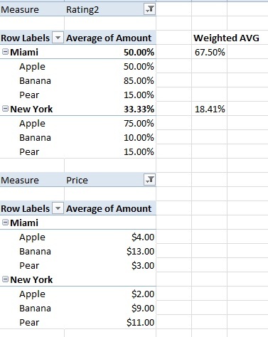
Obviously the weighted average of the Rating is different than the regular average. Is there a way to get the weighted averages in the sum fields? I don't even need the Apple, Banana and Pear in the columns, in the end what I want to achieve is just show the cities (New York, Miami) and their weighted averages.

Thanks,

Robert

 

[Mackers]

Hi Robert

So that we can help, could you provide some more information so I can tell exactly what you're hoping for. Are you trying to average the percentage, perhaps in order to spread the produce out as much as possible? If so, how are you calculating the weighted average? If it is by cost, I can't match your figures. Looking at Miami, 50% apples at $4 is $2, 85% bananas at $13 is $11.05 and 15% pears at $3 is $0.45. If you then find the percentage spend on each of these, i.e. divide $2 by the sum of the three weighted figures (being 13.5), divide 11.05 by 13.5 and divide 0.45 by 13.5 you get 14.8%, 81.8% and 0.03%. Averaging this is 33.33%. I might be getting confused about what it is you want here - giving an idea of what the "Rating" means might help

As an initial point, and I'm sure you've heard this before, I would suggest that you change your data structure. It makes more sense to have one column for Price and a separate column for Rating rather than a column specifying what another column refers to. This is just good practice - it keeps your results for each city/fruit combination on one row, it keeps your columns referring to the same thing, it makes 'missing' rows more obvious (e.g. you have the price but not the amount) and it keeps the data type the same in each column rather than having currency and percentages mixed up. If changing your data structure is not possible (why?), a solution would be to actually have a separate sheet that uses formulas to pull through this information using SUMIFS() into a proper structure. For example,

=SUMIFS(D2:D13,A2:A13,"Miami",B2:B13,"Apple",C2:C13,"Price")

Replace Miami, Apple and Price with cell references and input all of the unique combinations and you should end up with a decent looking data set.

Hope that helps

Mackers