Hello all,
I need help to find a way to use the Small+If structure with multiple criteria inside the If (without creating multiple If).
Currently my model works just fine if I have only one argument inside my If. For instance:
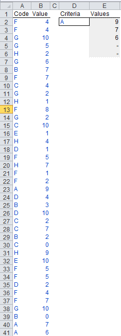
In here, the range E2:E6 is returning the values that match the criteria A (which are in row 23, 40 and 41).
The formula in cell E2 is (entered as an array): =IFERROR(SMALL(IF($A$1:$A$41=D$2,$B$1:$B$41,"-"),COUNTIF($A:$A,$D$2)-(ROW()-ROW($C$2))),"-")
Now, this worked just fine so far - but now I need to evolve it a little. Suppose that instead of A as an argument, I want it to return all the results that match A, B, C, D and E. I want to avoid as much as possible the use of multiple Ifs inside Ifs. I also want to avoid VBAs on this one.
Thoughts?
Thanks for the help!
Ps: I'll paste here the contents of columns A and B in case you want to give it a shot and recreate it in your Excel (sorry, I don't know how to edit the table in here and I don't have permissions to install the .exe file to edit tables)
Code Value
F 4
F 4
G 10
G 5
H 2
G 6
B 7
F 7
C 4
G 2
H 1
F 8
G 2
C 10
E 1
H 4
D 1
F 5
H 7
F 1
F 2
A 9
D 4
B 3
D 10
C 2
C 7
B 2
C 0
H 9
E 10
F 5
F 5
D 2
F 4
F 7
G 10
B 0
A 7
A 6
I need help to find a way to use the Small+If structure with multiple criteria inside the If (without creating multiple If).
Currently my model works just fine if I have only one argument inside my If. For instance:
In here, the range E2:E6 is returning the values that match the criteria A (which are in row 23, 40 and 41).
The formula in cell E2 is (entered as an array): =IFERROR(SMALL(IF($A$1:$A$41=D$2,$B$1:$B$41,"-"),COUNTIF($A:$A,$D$2)-(ROW()-ROW($C$2))),"-")
Now, this worked just fine so far - but now I need to evolve it a little. Suppose that instead of A as an argument, I want it to return all the results that match A, B, C, D and E. I want to avoid as much as possible the use of multiple Ifs inside Ifs. I also want to avoid VBAs on this one.
Thoughts?
Thanks for the help!
Ps: I'll paste here the contents of columns A and B in case you want to give it a shot and recreate it in your Excel (sorry, I don't know how to edit the table in here and I don't have permissions to install the .exe file to edit tables)
Code Value
F 4
F 4
G 10
G 5
H 2
G 6
B 7
F 7
C 4
G 2
H 1
F 8
G 2
C 10
E 1
H 4
D 1
F 5
H 7
F 1
F 2
A 9
D 4
B 3
D 10
C 2
C 7
B 2
C 0
H 9
E 10
F 5
F 5
D 2
F 4
F 7
G 10
B 0
A 7
A 6


